Matrix calculation with NumPy

23 of april of 2021

Disclaimer: This post has been translated to English using a machine translation model. Please, let me know if you find any mistakes.

1. Summary

Let's take a brief introduction to the matrix calculation library NumPy. This library is designed for all kinds of matrix calculations, so we will focus only on the part that will be useful for understanding the calculations within neural networks, but we will leave out interesting things like using the library for linear algebra.

2. What is NumPy?

NumPy is a Python library designed for performing matrix calculations. Matrix calculation is something that is widely used in science in general and in data science in particular, which is why it is necessary to have a library that does this very well.

Its name means Numerical Python

Its main object is the ndarray, which encapsulates n-dimensional arrays of homogeneous data types, unlike Python lists, which can have data of different types.

NumPy aims to perform matrix calculations much faster than with Python lists, but how is this possible?

NumPy uses compiled code, while Python uses interpreted code. The difference is that Python has to interpret, compile, and execute the code at runtime, whereas NumPy is already compiled, so it runs faster.
The ndarrays have a fixed size, unlike Python lists which are dynamic. If in NumPy you want to modify the size of an array, a new one will be created and the old one will be deleted.
All elements of ndarrays are of the same data type, unlike Python lists which can have elements of different types
Part of the NumPy code is written in C/C++ (much faster than Python)
The data in arrays is stored in memory continuously, unlike Python lists, which makes them much faster to manipulate

NumPy offers the convenience of using code that is easy to write and read, but it is written and precompiled in C, which makes it much faster.

Suppose we want to multiply two vectors, this would be done in C as follows:

for (i = 0; i < rows; i++): {
  for (j = 0; j < columns; j++): {
    c[i][j] = a[i][j]*b[i][j];
  }
}

NumPy offers the possibility of running this code under the hood, but in a much easier way to write and understand through

c = a * b

NumPy offers vectorized code, which means you don't have to write loops, but they are still being executed underneath in optimized and precompiled C code. This has the following advantages:

The code is easier to write and read
With fewer lines of code required, there is a lower chance of introducing errors
The code looks more like mathematical notation

2.1. NumPy as `np`

Generally, when importing NumPy, it is usually imported with the alias np

	
		
			< >
			Input
		
		
			Python
			
		
	
	
		import numpy as np
 
print(np.__version__)
	
	Copied

>_ Output

			
				1.18.1

3. Speed of NumPy

As explained, NumPy performs calculations much faster than Python lists. Let's look at an example where the dot product of two matrices is performed using Python lists and using ndarrays.

	
		
			< >
			Input
		
		
			Python
			
		
	
	
		from time import time
 
# Dimensión de las matrices
dim = 1000
shape = (dim, dim)
 
# Se crean dos ndarrays de NumPy de dimensión dim x dim
ndarray_a = np.ones(shape=shape)
ndarray_b = np.ones(shape=shape)
 
# Se crean dos listas de Python de dimensión dim x dim a partir de los ndarrays
list_a = list(ndarray_a)
list_b = list(ndarray_b)
 
# Se crean el ndarray y la lista de Python donde se guardarán los resultados
ndarray_c = np.empty(shape=shape)
list_c = list(ndarray_c)
 
# Producto escalar de dos listas de python
t0 = time()
for fila in range(dim):
  for columna in range(dim):
    list_c[fila][columna] = list_a[fila][columna] * list_b[fila][columna]
t = time()
t_listas = t-t0
print(f"Tiempo para realizar el producto escalar de dos listas de Python de dimensiones {dim}x{dim}: {t_listas:.4f} ms")
 
 
# Producto escalar de dos ndarrays de NumPy
t0 = time()
ndarray_c = ndarray_a * ndarray_b
t = time()
t_ndarrays = t-t0
print(f"Tiempo para realizar el producto escalar de dos ndarrays de NumPy de dimensiones {dim}x{dim}: {t_ndarrays:.4f} ms")
 
# Comparación de tiempos
print(f"
Hacer el cálculo con listas de Python tarda {t_listas/t_ndarrays:.2f} veces más rápido que con ndarrays de NumPy")
	
	Copied

>_ Output

			
				Tiempo para realizar el producto escalar de dos listas de Python de dimensiones 1000x1000: 0.5234 ms
Tiempo para realizar el producto escalar de dos ndarrays de NumPy de dimensiones 1000x1000: 0.0017 ms
Hacer el cálculo con listas de Python tarda 316.66 veces más rápido que con ndarrays de NumPy

4. Matrices in NumPy

In NumPy an array is an ndarray object

	
		
			< >
			Input
		
		
			Python
			
		
	
	
		arr = np.array([1, 2, 3, 4, 5])
 
print(arr)
print(type(arr))
	
	Copied

>_ Output

			
				[1 2 3 4 5]
&lt;class 'numpy.ndarray'&gt;

4.1. How to create arrays

With the array() method, you can create ndarrays by passing in Python lists (like in the previous example) or tuples.

	
		
			< >
			Input
		
		
			Python
			
		
	
	
		arr = np.array((1, 2, 3, 4, 5))
 
print(arr)
print(type(arr))
	
	Copied

>_ Output

			
				[1 2 3 4 5]
&lt;class 'numpy.ndarray'&gt;

With the zeros() method, you can create matrices filled with zeros

	
		
			< >
			Input
		
		
			Python
			
		
	
	
		arr = np.zeros((3, 4))
 
print(arr)
	
	Copied

>_ Output

			
				[[0. 0. 0. 0.]
[0. 0. 0. 0.]
[0. 0. 0. 0.]]

The method zeros_like(A) returns a matrix with the same shape as matrix A, but filled with zeros.

	
		
			< >
			Input
		
		
			Python
			
		
	
	
		A = np.array((1, 2, 3, 4, 5))
arr = np.zeros_like(A)
 
print(arr)
	
	Copied

>_ Output

			
				[0 0 0 0 0]

With the ones() method, you can create matrices filled with ones

	
		
			< >
			Input
		
		
			Python
			
		
	
	
		arr = np.ones((4, 3))
 
print(arr)
	
	Copied

>_ Output

			
				[[1. 1. 1.]
[1. 1. 1.]
[1. 1. 1.]
[1. 1. 1.]]

The method ones_like(A) returns an array with the same shape as array A, but filled with ones.

	
		
			< >
			Input
		
		
			Python
			
		
	
	
		A = np.array((1, 2, 3, 4, 5))
arr = np.ones_like(A)
 
print(arr)
	
	Copied

>_ Output

			
				[1 1 1 1 1]

With the empty() method, you can create arrays with the dimensions you desire, but they are initialized randomly.

	
		
			< >
			Input
		
		
			Python
			
		
	
	
		arr = np.empty((6, 3))
 
print(arr)
	
	Copied

>_ Output

			
				[[4.66169180e-310 2.35541533e-312 2.41907520e-312]
[2.14321575e-312 2.46151512e-312 2.31297541e-312]
[2.35541533e-312 2.05833592e-312 2.22809558e-312]
[2.56761491e-312 2.48273508e-312 2.05833592e-312]
[2.05833592e-312 2.29175545e-312 2.07955588e-312]
[2.14321575e-312 0.00000000e+000 0.00000000e+000]]

The method empty_like(A) returns an array with the same shape as array A, but initialized randomly.

	
		
			< >
			Input
		
		
			Python
			
		
	
	
		A = np.array((1, 2, 3, 4, 5))
arr = np.empty_like(A)
 
print(arr)
	
	Copied

>_ Output

			
				[4607182418800017408 4611686018427387904 4613937818241073152
4616189618054758400 4617315517961601024]

With the method arange(start, stop, step) you can create arrays within a specified range. This method is similar to Python's range() method.

	
		
			< >
			Input
		
		
			Python
			
		
	
	
		arr = np.arange(10, 30, 5)
 
print(arr)
	
	Copied

>_ Output

			
				[10 15 20 25]

When arange is used with floating-point arguments, it is generally not possible to predict the number of elements obtained, due to the finite precision of floating-point numbers.

For this reason, it is usually better to use the function linspace(start, stop, n) which takes as an argument the number of elements we want, instead of the step.

	
		
			< >
			Input
		
		
			Python
			
		
	
	
		arr = np.linspace(0, 2, 9)
 
print(arr)
	
	Copied

>_ Output

			
				[0.   0.25 0.5  0.75 1.   1.25 1.5  1.75 2.  ]

Lastly, if we want to create matrices with random numbers, we can use the random.rand function with a tuple containing the dimensions as a parameter.

	
		
			< >
			Input
		
		
			Python
			
		
	
	
		arr = np.random.rand(2, 3)
 
print(arr)
	
	Copied

>_ Output

			
				[[0.32726085 0.65571767 0.73126697]
[0.91938206 0.9862451  0.95033649]]

4.2. Matrix Dimensions

In NumPy we can create arrays of any dimension. To get the dimension of an array we use the ndim method.

Matrix of dimension 0, which would be equivalent to a number

	
		
			< >
			Input
		
		
			Python
			
		
	
	
		arr = np.array(42)
 
print(arr)
print(arr.ndim)
	
	Copied

>_ Output

			
				42
0

1-dimensional matrix, which would be equivalent to a vector

	
		
			< >
			Input
		
		
			Python
			
		
	
	
		arr = np.array([1, 2, 3, 4, 5])
 
print(arr)
print(arr.ndim)
	
	Copied

>_ Output

			
				[1 2 3 4 5]
1

2-dimensional matrix, which would be equivalent to a matrix

	
		
			< >
			Input
		
		
			Python
			
		
	
	
		arr = np.array([[1, 2, 3, 4, 5],
                [6, 7, 8, 9, 10]])
 
print(arr)
print(arr.ndim)
	
	Copied

>_ Output

			
				[[ 1  2  3  4  5]
[ 6  7  8  9 10]]
2

Matrix of dimension 3

	
		
			< >
			Input
		
		
			Python
			
		
	
	
		arr = np.array([
                [[1, 2, 3, 4, 5],
                [6, 7, 8, 9, 10]],
                
                [[11, 12, 13, 14, 15],
                [16, 17, 18, 19, 20]]
                ])
 
print(arr)
print(arr.ndim)
	
	Copied

>_ Output

			
				[[[ 1  2  3  4  5]
  [ 6  7  8  9 10]]
[[11 12 13 14 15]
  [16 17 18 19 20]]]
3

Matrix of dimension N. When creating ndarrays, the number of dimensions can be set using the ndim parameter.

	
		
			< >
			Input
		
		
			Python
			
		
	
	
		arr = np.array([1, 2, 3, 4, 5], ndmin=6)
 
print(arr)
print(arr.ndim)
	
	Copied

>_ Output

			
				[[[[[[1 2 3 4 5]]]]]]
6

4.3. Size of the matrices

If we want to see the size of the matrix instead of its dimension, we can use the shape method.

	
		
			< >
			Input
		
		
			Python
			
		
	
	
		arr = np.array([
                [[1, 2, 3, 4, 5],
                [6, 7, 8, 9, 10]],
                
                [[11, 12, 13, 14, 15],
                [16, 17, 18, 19, 20]]
                ])
 
print(arr.shape)
	
	Copied

>_ Output

			
				(2, 2, 5)

5. Data Types

The data that NumPy arrays can store are the following:

i - integer
b - boolean
u - unsigned integer
f - float
c - Complex floating point
m - Timedelta
M - DateTime
O - Object
S - string
U - Unicode string
V - Fixed memory fragment for another type (void)

We can check the data type of an array using dtype

	
		
			< >
			Input
		
		
			Python
			
		
	
	
		arr = np.array([1, 2, 3, 4])
print(arr.dtype)
 
arr = np.array(['apple', 'banana', 'cherry'])
print(arr.dtype)
	
	Copied

>_ Output

			
				int64
&lt;U6

We can also create arrays specifying the data type we want them to have using dtype

	
		
			< >
			Input
		
		
			Python
			
		
	
	
		arr = np.array([1, 2, 3, 4], dtype='i')
print("Enteros:")
print(arr)
print(arr.dtype)
 
arr = np.array([1, 2, 3, 4], dtype='f')
print("
Float:")
print(arr)
print(arr.dtype)
 
arr = np.array([1, 2, 3, 4], dtype='f')
print("
Complejos:")
print(arr)
print(arr.dtype)
 
arr = np.array([1, 2, 3, 4], dtype='S')
print("
String:")
print(arr)
print(arr.dtype)
 
arr = np.array([1, 2, 3, 4], dtype='U')
print("
Unicode string:")
print(arr)
print(arr.dtype)
 
arr = np.array([1, 2, 3, 4], dtype='O')
print("
Objeto:")
print(arr)
print(arr.dtype)
	
	Copied

>_ Output

			
				Enteros:
[1 2 3 4]
int32
Float:
[1. 2. 3. 4.]
float32
Complejos:
[1. 2. 3. 4.]
float32
String:
[b'1' b'2' b'3' b'4']
|S1
Unicode string:
['1' '2' '3' '4']
&lt;U1
Objeto:
[1 2 3 4]
object

6. Mathematical Operations

6.1. Basic Operations

Matrix operations are performed element-wise, for example, if we add two matrices, the elements of each matrix in the same position will be added, just as it is done in the mathematical addition of two matrices.

	
		
			< >
			Input
		
		
			Python
			
		
	
	
		A = np.array([1, 2, 3])
B = np.array([1, 2, 3])
 
print(f"Matriz A: tamaño {A.shape}
{A}
")
print(f"Matriz B: tamaño {B.shape}
{B}
")
 
C = A + B
print(f"Matriz C: tamaño {C.shape}
{C}
")
 
D = A - B
print(f"Matriz D: tamaño {D.shape}
{D}")
	
	Copied

>_ Output

			
				Matriz A: tamaño (3,)
[1 2 3]
Matriz B: tamaño (3,)
[1 2 3]
Matriz C: tamaño (3,)
[2 4 6]
Matriz D: tamaño (3,)
[0 0 0]

However, if we perform the multiplication of two matrices, the multiplication of each element of the matrices (dot product) is also carried out.

	
		
			< >
			Input
		
		
			Python
			
		
	
	
		A = np.array([[3, 5], [4, 1]])
B = np.array([[1, 2], [-3, 0]])
 
print(f"Matriz A: tamaño {A.shape}
{A}
")
print(f"Matriz B: tamaño {B.shape}
{B}
")
 
C = A * B
print(f"Matriz C: tamaño {C.shape}
{C}
")
	
	Copied

>_ Output

			
				Matriz A: tamaño (2, 2)
[[3 5]
[4 1]]
Matriz B: tamaño (2, 2)
[[ 1  2]
[-3  0]]
Matriz C: tamaño (2, 2)
[[  3  10]
[-12   0]]

To perform the matrix product that has been taught in mathematics all along, you have to use the operator @ or the method dot.

	
		
			< >
			Input
		
		
			Python
			
		
	
	
		A = np.array([[3, 5], [4, 1], [6, -1]])
B = np.array([[1, 2, 3], [-3, 0, 4]])
 
print(f"Matriz A: tamaño {A.shape}
{A}
")
print(f"Matriz B: tamaño {B.shape}
{B}
")
 
C = A @ B
print(f"Matriz C: tamaño {C.shape}
{C}
")
 
D = A.dot(B)
print(f"Matriz D: tamaño {D.shape}
{D}")
	
	Copied

>_ Output

			
				Matriz A: tamaño (3, 2)
[[ 3  5]
[ 4  1]
[ 6 -1]]
Matriz B: tamaño (2, 3)
[[ 1  2  3]
[-3  0  4]]
Matriz C: tamaño (3, 3)
[[-12   6  29]
[  1   8  16]
[  9  12  14]]
Matriz D: tamaño (3, 3)
[[-12   6  29]
[  1   8  16]
[  9  12  14]]

If instead of creating a new array, you want to modify an existing one, you can use the operators +=, -= or *=

	
		
			< >
			Input
		
		
			Python
			
		
	
	
		A = np.array([[3, 5], [4, 1]])
B = np.array([[1, 2], [-3, 0]])
 
print(f"Matriz A: tamaño {A.shape}
{A}
")
print(f"Matriz B: tamaño {B.shape}
{B}
")
 
A += B
print(f"Matriz A tras suma: tamaño {A.shape}
{A}
")
 
A -= B
print(f"Matriz A tras resta: tamaño {A.shape}
{A}
")
 
A *= B
print(f"Matriz A tras multiplicación: tamaño {A.shape}
{A}
")
	
	Copied

>_ Output

			
				Matriz A: tamaño (2, 2)
[[3 5]
[4 1]]
Matriz B: tamaño (2, 2)
[[ 1  2]
[-3  0]]
Matriz A tras suma: tamaño (2, 2)
[[4 7]
[1 1]]
Matriz A tras resta: tamaño (2, 2)
[[3 5]
[4 1]]
Matriz A tras multiplicación: tamaño (2, 2)
[[  3  10]
[-12   0]]

Operations can be performed on all elements of an array, thanks to a property called broadcasting, which we will explore in more detail later.

	
		
			< >
			Input
		
		
			Python
			
		
	
	
		A = np.array([[3, 5], [4, 1]])
 
print(f"Matriz A: tamaño {A.shape}
{A}
")
 
B = A * 2
print(f"Matriz B: tamaño {B.shape}
{B}
")
 
C = A ** 2
print(f"Matriz C: tamaño {C.shape}
{C}
")
 
D = 2*np.sin(A)
print(f"Matriz D: tamaño {D.shape}
{D}")
	
	Copied

>_ Output

			
				Matriz A: tamaño (2, 2)
[[3 5]
[4 1]]
Matriz B: tamaño (2, 2)
[[ 6 10]
[ 8  2]]
Matriz C: tamaño (2, 2)
[[ 9 25]
[16  1]]
Matriz D: tamaño (2, 2)
[[ 0.28224002 -1.91784855]
[-1.51360499  1.68294197]]

6.2. Functions on Matrices

As can be seen in the last calculation, NumPy offers function operators over arrays; there are a lot of functions that can be performed on arrays, such as mathematical, logical, linear algebra, etc. We show some below.

	
		
			< >
			Input
		
		
			Python
			
		
	
	
		A = np.array([[3, 5], [4, 1]])
 
print(f"A
{A}
")
 
print(f"exp(A)
{np.exp(A)}
")
print(f"sqrt(A)
{np.sqrt(A)}
")
print(f"cos(A)
{np.cos(A)}
")
	
	Copied

>_ Output

			
				A
[[3 5]
[4 1]]
exp(A)
[[ 20.08553692 148.4131591 ]
[ 54.59815003   2.71828183]]
sqrt(A)
[[1.73205081 2.23606798]
[2.         1.        ]]
cos(A)
[[-0.9899925   0.28366219]
[-0.65364362  0.54030231]]

There are some functions that return information about the arrays, such as the mean

	
		
			< >
			Input
		
		
			Python
			
		
	
	
		A = np.array([[3, 5], [4, 1]])
 
print(f"A
{A}
")
 
print(f"A.mean()
{A.mean()}
")
	
	Copied

>_ Output

			
				A
[[3 5]
[4 1]]
A.mean()
3.25

However, we can obtain such information for each axis through the axis attribute. If it is 0, it is done over each column; while if it is 1, it is done over each row.

	
		
			< >
			Input
		
		
			Python
			
		
	
	
		A = np.array([[3, 5], [4, 1]])
 
print(f"A
{A}
")
 
print(f"A.mean() columnas
{A.mean(axis=0)}
")
print(f"A.mean() filas
{A.mean(axis=1)}
")
	
	Copied

>_ Output

			
				A
[[3 5]
[4 1]]
A.mean() columnas
[3.5 3. ]
A.mean() filas
[4.  2.5]

6.3. Broadcasting

Matrix operations can be performed with matrices of different dimensions. In this case, NumPy will detect this and project the smaller matrix to match the larger one.

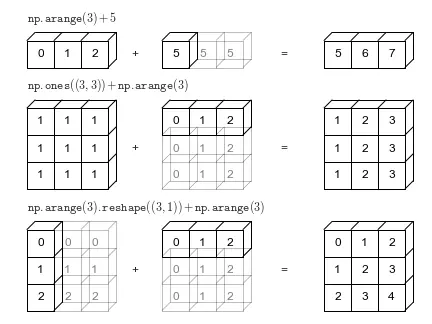
This is a great feature of NumPy, which allows calculations to be performed on arrays without having to worry about matching their dimensions.

	
		
			< >
			Input
		
		
			Python
			
		
	
	
		A = np.array([1, 2, 3])
 
print(f"A
{A}
")
 
B = A + 5
 
print(f"B
{B}
")
	
	Copied

>_ Output

			
				A
[1 2 3]
B
[6 7 8]

	
		
			< >
			Input
		
		
			Python
			
		
	
	
		A = np.array([1, 2, 3])
B = np.ones((3,3))
 
print(f"A
{A}
")
print(f"B
{B}
")
 
C = A + B
 
print(f"C
{C}
")
	
	Copied

>_ Output

			
				A
[1 2 3]
B
[[1. 1. 1.]
[1. 1. 1.]
[1. 1. 1.]]
C
[[2. 3. 4.]
[2. 3. 4.]
[2. 3. 4.]]

	
		
			< >
			Input
		
		
			Python
			
		
	
	
		A = np.array([1, 2, 3])
B = np.array([[1], [2], [3]])
 
print(f"A
{A}
")
print(f"B
{B}
")
 
C = A + B
 
print(f"C
{C}
")
	
	Copied

>_ Output

			
				A
[1 2 3]
B
[[1]
[2]
[3]]
C
[[2 3 4]
[3 4 5]
[4 5 6]]

7. Matrix Indexing

Matrix indexing is done the same way as with Python lists

	
		
			< >
			Input
		
		
			Python
			
		
	
	
		arr = np.array([1, 2, 3, 4, 5])
arr[3]
	
	Copied

>_ Output

In the case of having more than one dimension, the index must be specified for each of them.

	
		
			< >
			Input
		
		
			Python
			
		
	
	
		arr = np.array([[1, 2, 3, 4, 5],
                [6, 7, 8, 9, 10]])
arr[1, 2]
	
	Copied

>_ Output

Negative indexing can be used

	
		
			< >
			Input
		
		
			Python
			
		
	
	
		arr[-1, -2]
	
	Copied

>_ Output

If one of the axes is not specified, it is considered that the full axis is intended.

	
		
			< >
			Input
		
		
			Python
			
		
	
	
		arr = np.array([[1, 2, 3, 4, 5],
                [6, 7, 8, 9, 10]])
arr[1]
	
	Copied

>_ Output

			
				array([ 6,  7,  8,  9, 10])

7.1. Slices of arrays

When indexing, we can keep parts of arrays just like we did with Python lists.

Remember that it was done as follows:

start:stop:step

Where the range goes from start (inclusive) to stop (exclusive) with a step of step

If step is not specified, it defaults to 1

For example, if we want items from the second row and from the second to the fourth column:

We select the second row with a 1 (since counting starts from 0)
We select from the second to the fourth row using 1:4, where 1 indicates the second column and 4 indicates the fifth (since the second number specifies the column where it ends without including this column). Both numbers taking into account that counting starts from 0.

	
		
			< >
			Input
		
		
			Python
			
		
	
	
		print(arr)
print(arr[1, 1:4])
	
	Copied

>_ Output

			
				[[ 1  2  3  4  5]
[ 6  7  8  9 10]]
[7 8 9]

We can take from a position to the end

	
		
			< >
			Input
		
		
			Python
			
		
	
	
		arr[1, 2:]
	
	Copied

>_ Output

			
				array([ 8,  9, 10])

From the beginning to a position

	
		
			< >
			Input
		
		
			Python
			
		
	
	
		arr[1, :3]
	
	Copied

>_ Output

			
				array([6, 7, 8])

Set the range with negative numbers

	
		
			< >
			Input
		
		
			Python
			
		
	
	
		arr[1, -3:-1]
	
	Copied

>_ Output

			
				array([8, 9])

Choose the step

	
		
			< >
			Input
		
		
			Python
			
		
	
	
		arr[1, 1:4:2]
	
	Copied

>_ Output

			
				array([7, 9])

7.2. Iteration over arrays

Iteration over multidimensional arrays is performed with respect to the first axis.

	
		
			< >
			Input
		
		
			Python
			
		
	
	
		M = np.array( [[[ 0, 1, 2],
                [ 10, 12, 13]],
               [[100,101,102],
                [110,112,113]]])
 
print(f'Matriz de dimensión: {M.shape}
')
 
i = 0
for fila in M:
  print(f'Fila {i}: {fila}')
  i += 1
	
	Copied

>_ Output

			
				Matriz de dimensión: (2, 2, 3)
Fila 0: [[ 0  1  2]
[10 12 13]]
Fila 1: [[100 101 102]
[110 112 113]]

However, if what we want is to iterate over each item, we can use the 'flat' method

	
		
			< >
			Input
		
		
			Python
			
		
	
	
		i = 0
for fila in M.flat:
  print(f'Elemento {i}: {fila}')
  i += 1
	
	Copied

>_ Output

			
				Elemento 0: 0
Elemento 1: 1
Elemento 2: 2
Elemento 3: 10
Elemento 4: 12
Elemento 5: 13
Elemento 6: 100
Elemento 7: 101
Elemento 8: 102
Elemento 9: 110
Elemento 10: 112
Elemento 11: 113

8. Matrix Copying

In NumPy we have two ways to copy arrays: using copy, which makes a new copy of the array, and using view, which creates a view of the original array.

The copy owns the data and any changes made to the copy will not affect the original array, and any changes made to the original array will not affect the copy.

The view is not the owner of the data and any changes made to the copy will affect the original array, and any changes made to the original array will affect the copy.

8.1. Copy

	
		
			< >
			Input
		
		
			Python
			
		
	
	
		arr = np.array([1, 2, 3, 4, 5])
copy_arr = arr.copy()
arr[0] = 42
copy_arr[1] = 43
 
print(f'Original: {arr}')
print(f'Copia:    {copy_arr}')
	
	Copied

>_ Output

			
				Original: [42  2  3  4  5]
Copia:    [ 1 43  3  4  5]

8.2. View

	
		
			< >
			Input
		
		
			Python
			
		
	
	
		arr = np.array([1, 2, 3, 4, 5])
view_arr = arr.view()
arr[0] = 42
view_arr[1] = 43
 
print(f'Original: {arr}')
print(f'Vista:    {view_arr}')
	
	Copied

>_ Output

			
				Original: [42 43  3  4  5]
Vista:    [42 43  3  4  5]

8.3. Data Owner

In case of doubt whether we have a copy or a view, we can use base

	
		
			< >
			Input
		
		
			Python
			
		
	
	
		arr = np.array([1, 2, 3, 4, 5])
 
copy_arr = arr.copy()
view_arr = arr.view()
 
print(copy_arr.base)
print(view_arr.base)
	
	Copied

>_ Output

			
				None
[1 2 3 4 5]

9. Shape of Matrices

We can know the shape of the matrix using the shape method. This will return a tuple, the size of the tuple represents the dimensions of the matrix, and each element of the tuple indicates the number of items in each of the matrix's dimensions.

	
		
			< >
			Input
		
		
			Python
			
		
	
	
		arr = np.array([
                [[1, 2, 3, 4, 5],
                [6, 7, 8, 9, 10]],
                
                [[11, 12, 13, 14, 15],
                [16, 17, 18, 19, 20]]
                ])
 
print(arr)
print(arr.shape)
	
	Copied

>_ Output

			
				[[[ 1  2  3  4  5]
  [ 6  7  8  9 10]]
[[11 12 13 14 15]
  [16 17 18 19 20]]]
(2, 2, 5)

9.1. Reshape

We can change the shape of the arrays to whatever we want using the reshape method.

For example, the previous matrix, which has a shape of (2, 2, 4). We can reshape it to (5, 4).

	
		
			< >
			Input
		
		
			Python
			
		
	
	
		arr_reshape = arr.reshape(5, 4)
 
print(arr_reshape)
print(arr_reshape.shape)
	
	Copied

>_ Output

			
				[[ 1  2  3  4]
[ 5  6  7  8]
[ 9 10 11 12]
[13 14 15 16]
[17 18 19 20]]
(5, 4)

It is important to note that when resizing arrays, the number of items in the new shape must match the number of items in the original shape.

That is, in the previous example, the first array had 20 items (2x2x4), and the new array has 20 items (5x4). What we cannot do is resize it to an array of size (3, 4), since there would be a total of 12 items.

	
		
			< >
			Input
		
		
			Python
			
		
	
	
		arr_reshape = arr.reshape(3, 4)
	
	Copied

>_ Output

			
				---------------------------------------------------------------------------ValueError                                Traceback (most recent call last)&lt;ipython-input-12-29e85875d1df&gt; in &lt;module&gt;()
----&gt; 1 arr_reshape = arr.reshape(3, 4)
ValueError: cannot reshape array of size 20 into shape (3,4)

9.2. Unknown Dimension

In the case where we want to change the shape of an array and one of the dimensions is irrelevant or unknown, we can have NumPy calculate it for us by passing a -1 as the parameter.

	
		
			< >
			Input
		
		
			Python
			
		
	
	
		arr = np.array([
                [[1, 2, 3, 4, 5],
                [6, 7, 8, 9, 10]],
                
                [[11, 12, 13, 14, 15],
                [16, 17, 18, 19, 20]]
                ])
 
arr_reshape = arr.reshape(2, -1)
 
print(arr_reshape)
print(arr_reshape.shape)
	
	Copied

>_ Output

			
				[[ 1  2  3  4  5  6  7  8  9 10]
[11 12 13 14 15 16 17 18 19 20]]
(2, 10)

It's important to note that you can't put any number in the known dimensions. The number of items in the original matrix must be a multiple of the known dimensions.

In the previous example, the array has 20 items, which is a multiple of 2, the known dimension introduced. A 3 could not have been used as the known dimension, since 20 is not a multiple of 3, and there would be no number that could be placed in the unknown dimension to make the total number of items 20.

9.3. Flattening of Matrices

We can flatten the arrays, that is, convert them to a single dimension using reshape(-1). This way, regardless of the dimensions of the original array, the new one will always have a single dimension.

	
		
			< >
			Input
		
		
			Python
			
		
	
	
		arr = np.array([
                [[1, 2, 3, 4, 5],
                [6, 7, 8, 9, 10]],
                
                [[11, 12, 13, 14, 15],
                [16, 17, 18, 19, 20]]
                ])
 
arr_flatten = arr.reshape(-1)
 
print(arr_flatten)
print(arr_flatten.shape)
	
	Copied

>_ Output

			
				[ 1  2  3  4  5  6  7  8  9 10 11 12 13 14 15 16 17 18 19 20]
(20,)

Another way to flatten an array is through the ravel() method.

	
		
			< >
			Input
		
		
			Python
			
		
	
	
		arr = np.array([
                [[1, 2, 3, 4, 5],
                [6, 7, 8, 9, 10]],
                
                [[11, 12, 13, 14, 15],
                [16, 17, 18, 19, 20]]
                ])
 
arr_flatten = arr.ravel()
 
print(arr_flatten)
print(arr_flatten.shape)
	
	Copied

>_ Output

			
				[ 1  2  3  4  5  6  7  8  9 10 11 12 13 14 15 16 17 18 19 20]
(20,)

9.4. Transpose Matrix

The transpose of a matrix can be obtained using the method T. Transposing a matrix means swapping its rows and columns. The following image provides an example that clarifies this further.

	
		
			< >
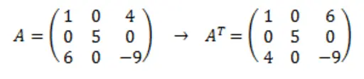
			Input
		
		
			Python
			
		
	
	
		arr = np.array([[1, 0, 4],
                [0, 5, 0],
                [6, 0, -9]])
 
arr_t = arr.T
 
print(arr_t)
print(arr_t.shape)
	
	Copied

>_ Output

			
				[[ 1  0  6]
[ 0  5  0]
[ 4  0 -9]]
(3, 3)

10. Stacking of Matrices

10.1. Vertical Stacking

Matrices can be stacked vertically (by joining rows) using the vstack() method.

	
		
			< >
			Input
		
		
			Python
			
		
	
	
		a = np.array([[1, 1, 1],
              [2, 2, 2],
              [3, 3, 3]])
 
b = np.array([[4, 4, 4],
              [5, 5, 5],
              [6, 6, 6]])
 
c = np.vstack((a,b))
c
	
	Copied

>_ Output

			
				array([[1, 1, 1],
       [2, 2, 2],
       [3, 3, 3],
       [4, 4, 4],
       [5, 5, 5],
       [6, 6, 6]])

If you have matrices with more than 2 dimensions, vstack() will stack along the first dimension

	
		
			< >
			Input
		
		
			Python
			
		
	
	
		a = np.array([
                [[1, 1],
                [2, 2]],
                
                [[3, 3],
                [4, 4]]
                ])
 
b = np.array([
                [[5, 5],
                [6, 6]],
                
                [[7, 7],
                [8, 8]]
                ])
 
c = np.vstack((a,b))
c
	
	Copied

>_ Output

			
				array([[[1, 1],
        [2, 2]],
       [[3, 3],
        [4, 4]],
       [[5, 5],
        [6, 6]],
       [[7, 7],
        [8, 8]]])

10.2. Horizontal Stacking

Matrices can be stacked horizontally (joining columns) using the hstack() method.

	
		
			< >
			Input
		
		
			Python
			
		
	
	
		a = np.array([[1, 2, 3],
              [1, 2, 3],
              [1, 2, 3]])
 
b = np.array([[4, 5, 6],
              [4, 5, 6],
              [4, 5, 6]])
 
c = np.hstack((a,b))
c
	
	Copied

>_ Output

			
				array([[1, 2, 3, 4, 5, 6],
       [1, 2, 3, 4, 5, 6],
       [1, 2, 3, 4, 5, 6]])

If you have matrices with more than 2 dimensions, hstack() will stack along the second dimension.

	
		
			< >
			Input
		
		
			Python
			
		
	
	
		a = np.array([
                [[1, 1],
                [2, 2]],
                
                [[3, 3],
                [4, 4]]
                ])
 
b = np.array([
                [[5, 5],
                [6, 6]],
                
                [[7, 7],
                [8, 8]]
                ])
 
c = np.hstack((a,b))
c
	
	Copied

>_ Output

			
				array([[[1, 1],
        [2, 2],
        [5, 5],
        [6, 6]],
       [[3, 3],
        [4, 4],
        [7, 7],
        [8, 8]]])

Another way to add columns to an array is by using the column_stack() method.

	
		
			< >
			Input
		
		
			Python
			
		
	
	
		a = np.array([[1, 2, 3],
              [1, 2, 3],
              [1, 2, 3]])
 
b = np.array([4, 4, 4])
 
c = np.column_stack((a,b))
c
	
	Copied

>_ Output

			
				array([[1, 2, 3, 4],
       [1, 2, 3, 4],
       [1, 2, 3, 4]])

10.3. Depth Stacking

Matrices can be stacked in depth (third dimension) using the dstack() method.

	
		
			< >
			Input
		
		
			Python
			
		
	
	
		a = np.array([
                [[1, 1],
                [2, 2]],
                
                [[3, 3],
                [4, 4]]
                ])
 
b = np.array([
                [[1, 1],
                [2, 2]],
                
                [[3, 3],
                [4, 4]]
                ])
 
c = np.dstack((a,b))
print(f"c: {c}
")
print(f"a.shape: {a.shape}, b.shape: {b.shape}, c.shape: {c.shape}")
	
	Copied

>_ Output

			
				c: [[[1 1 1 1]
  [2 2 2 2]]
[[3 3 3 3]
  [4 4 4 4]]]
a.shape: (2, 2, 2), b.shape: (2, 2, 2), c.shape: (2, 2, 4)

If you have matrices with more than 4 dimensions, dstack() will stack along the third dimension.

	
		
			< >
			Input
		
		
			Python
			
		
	
	
		a = np.array([1, 2, 3, 4, 5], ndmin=4)
 
b = np.array([1, 2, 3, 4, 5], ndmin=4)
 
c = np.dstack((a,b))
print(f"a.shape: {a.shape}, b.shape: {b.shape}, c.shape: {c.shape}")
	
	Copied

>_ Output

			
				a.shape: (1, 1, 1, 5), b.shape: (1, 1, 1, 5), c.shape: (1, 1, 2, 5)

10.3. Custom Stacking

Using the concatenate() method, you can choose the axis along which the arrays should be stacked.

	
		
			< >
			Input
		
		
			Python
			
		
	
	
		a = np.array([
                [[1, 1],
                [2, 2]],
                
                [[3, 3],
                [4, 4]]
                ])
 
b = np.array([
                [[5, 5],
                [6, 6]],
                
                [[7, 7],
                [8, 8]]
                ])
 
conc0 = np.concatenate((a,b), axis=0) # concatenamiento en el primer eje
conc1 = np.concatenate((a,b), axis=1) # concatenamiento en el segundo eje
conc2 = np.concatenate((a,b), axis=2) # concatenamiento en el tercer eje
print(f"conc0: {conc0}
")
print(f"conc1: {conc1}
")
print(f"conc2: {conc2}")
	
	Copied

>_ Output

			
				conc0: [[[1 1]
  [2 2]]
[[3 3]
  [4 4]]
[[5 5]
  [6 6]]
[[7 7]
  [8 8]]]
conc1: [[[1 1]
  [2 2]
  [5 5]
  [6 6]]
[[3 3]
  [4 4]
  [7 7]
  [8 8]]]
conc2: [[[1 1 5 5]
  [2 2 6 6]]
[[3 3 7 7]
  [4 4 8 8]]]

11. Splitting Arrays

11.1. Split Vertically

Matrices can be divided vertically (separating rows) using the vsplit() method.

	
		
			< >
			Input
		
		
			Python
			
		
	
	
		a = np.array([[1.1, 1.2, 1.3, 1.4],
              [2.1, 2.2, 2.3, 2.4],
              [3.1, 3.2, 3.3, 3.4],
              [4.1, 4.2, 4.3, 4.4]])
 
[a1, a2] = np.vsplit(a, 2)
print(f"a1: {a1}
")
print(f"a2: {a2}")
	
	Copied

>_ Output

			
				a1: [[1.1 1.2 1.3 1.4]
[2.1 2.2 2.3 2.4]]
a2: [[3.1 3.2 3.3 3.4]
[4.1 4.2 4.3 4.4]]

If you have matrices with more than 2 dimensions, vsplit() will split along the first dimension.

	
		
			< >
			Input
		
		
			Python
			
		
	
	
		a = np.array([
                [[1, 1],
                [2, 2]],
                
                [[3, 3],
                [4, 4]]
                ])
 
[a1, a2] = np.vsplit(a, 2)
print(f"a1: {a1}
")
print(f"a2: {a2}")
	
	Copied

>_ Output

			
				a1: [[[1 1]
  [2 2]]]
a2: [[[3 3]
  [4 4]]]

11.2. Split Horizontally

Matrices can be split horizontally (separating columns) using the hsplit() method.

	
		
			< >
			Input
		
		
			Python
			
		
	
	
		a = np.array([[1.1, 1.2, 1.3, 1.4],
              [2.1, 2.2, 2.3, 2.4],
              [3.1, 3.2, 3.3, 3.4],
              [4.1, 4.2, 4.3, 4.4]])
 
[a1, a2] = np.hsplit(a, 2)
print(f"a1: {a1}
")
print(f"a2: {a2}")
	
	Copied

>_ Output

			
				a1: [[1.1 1.2]
[2.1 2.2]
[3.1 3.2]
[4.1 4.2]]
a2: [[1.3 1.4]
[2.3 2.4]
[3.3 3.4]
[4.3 4.4]]

If you have matrices with more than 2 dimensions, hsplit() will split along the second dimension

	
		
			< >
			Input
		
		
			Python
			
		
	
	
		a = np.array([
                [[1, 1],
                [2, 2]],
                
                [[3, 3],
                [4, 4]]
                ])
 
[a1, a2] = np.hsplit(a, 2)
print(f"a1: {a1}
")
print(f"a2: {a2}")
	
	Copied

>_ Output

			
				a1: [[[1 1]]
[[3 3]]]
a2: [[[2 2]]
[[4 4]]]

11.3. Custom Splitting

Using the array_split() method, you can choose the axis along which to split the arrays.

	
		
			< >
			Input
		
		
			Python
			
		
	
	
		a = np.array([
                [[1, 1],
                [2, 2]],
                
                [[3, 3],
                [4, 4]]
                ])
 
[a1_eje0, a2_eje0] = np.array_split(a, 2, axis=0)
[a1_eje1, a2_eje1] = np.array_split(a, 2, axis=1)
[a1_eje2, a2_eje2] = np.array_split(a, 2, axis=2)
 
print(f"a1_eje0: {a1_eje0}
")
print(f"a2_eje0: {a2_eje0}

")
 
print(f"a1_eje1: {a1_eje1}
")
print(f"a2_eje1: {a2_eje1}

")
 
print(f"a1_eje2: {a1_eje2}
")
print(f"a2_eje2: {a2_eje2}")
	
	Copied

>_ Output

			
				a1_eje0: [[[1 1]
  [2 2]]]
a2_eje0: [[[3 3]
  [4 4]]]
a1_eje1: [[[1 1]]
[[3 3]]]
a2_eje1: [[[2 2]]
[[4 4]]]
a1_eje2: [[[1]
  [2]]
[[3]
  [4]]]
a2_eje2: [[[1]
  [2]]
[[3]
  [4]]]

12. Matrix Search

If you want to search for a value within an array, you can use the where() method which returns the positions where the array has the value we are looking for.

	
		
			< >
			Input
		
		
			Python
			
		
	
	
		arr = np.array([1, 2, 3, 4, 5, 4, 4])
 
ids = np.where(arr == 4)
ids
	
	Copied

>_ Output

			
				(array([3, 5, 6]),)

Functions can be used to search, for example, if we want to find the positions where the values are even.

	
		
			< >
			Input
		
		
			Python
			
		
	
	
		arr = np.array([1, 2, 3, 4, 5, 6, 7, 8])
 
ids = np.where(arr%2)
ids
	
	Copied

>_ Output

			
				(array([0, 2, 4, 6]),)

13. Sorting Arrays

By using the sort() method, we can sort arrays

	
		
			< >
			Input
		
		
			Python
			
		
	
	
		arr = np.array([3, 2, 0, 1])
 
arr_ordenado = np.sort(arr)
arr_ordenado
	
	Copied

>_ Output

			
				array([0, 1, 2, 3])

If we have strings, it sorts them alphabetically

	
		
			< >
			Input
		
		
			Python
			
		
	
	
		arr = np.array(['banana', 'apple', 'cherry'])
 
arr_ordenado = np.sort(arr)
arr_ordenado
	
	Copied

>_ Output

			
				array(['apple', 'banana', 'cherry'], dtype='&lt;U6')

And it also sorts boolean arrays.

	
		
			< >
			Input
		
		
			Python
			
		
	
	
		arr = np.array([True, False, True])
 
arr_ordenado = np.sort(arr)
arr_ordenado
	
	Copied

>_ Output

			
				array([False,  True,  True])

If you have matrices with more than one dimension, it sorts them by dimensions, that is, if you have a 2-dimensional matrix, it sorts the numbers in the first row among themselves and those in the second row among themselves.

	
		
			< >
			Input
		
		
			Python
			
		
	
	
		arr = np.array([[3, 2, 4], [5, 0, 1]])
 
arr_ordenado = np.sort(arr)
arr_ordenado
	
	Copied

>_ Output

			
				array([[2, 3, 4],
       [0, 1, 5]])

By default, it sorts always with respect to the rows, but if you want it to sort with respect to another dimension, you have to specify it through the axis variable.

	
		
			< >
			Input
		
		
			Python
			
		
	
	
		arr = np.array([[3, 2, 4], [5, 0, 1]])
 
arr_ordenado0 = np.sort(arr, axis=0) # Se ordena con respecto a la primera dimensión
arr_ordenado1 = np.sort(arr, axis=1) # Se ordena con respecto a la segunda dimensión
 
print(f"arr_ordenado0: {arr_ordenado0}
")
print(f"arr_ordenado1: {arr_ordenado1}
")
	
	Copied

>_ Output

			
				arr_ordenado0: [[3 0 1]
[5 2 4]]
arr_ordenado1: [[2 3 4]
[0 1 5]]

14. Filters in arrays

NumPy offers the possibility to search for certain elements in an array and create a new one

This is done by creating a boolean index array, that is, it creates a new array that indicates which positions we keep from the original array and which ones we do not.

Let's look at an example of a boolean index matrix

	
		
			< >
			Input
		
		
			Python
			
		
	
	
		arr = np.array([37, 85, 12, 45, 69, 22])
 
indices_booleanos = [False, False, True, False, False, True]
 
arr_filter = arr[indices_booleanos]
 
print(f"Array original: {arr}")
print(f"indices booleanos: {indices_booleanos}")
print(f"Array filtrado: {arr_filter}")
	
	Copied

>_ Output

			
				Array original: [37 85 12 45 69 22]
indices booleanos: [False, False, True, False, False, True]
Array filtrado: [12 22]

As can be seen, the filtered array (arr_filtr), only retains the elements from the original array (arr) that correspond to those where the array indices_booleanos is True

Another thing we can see is that it has only kept the even elements, so now we will look at how to keep the even elements of an array without having to do it by hand as we did in the previous example.

	
		
			< >
			Input
		
		
			Python
			
		
	
	
		arr = np.array([[1, 2, 3, 4, 5],
                [6, 7, 8, 9, 10]])
 
indices_booleanos = arr % 2 == 0
 
arr_filter = arr[indices_booleanos]
 
print(f"Array original: {arr}
")
print(f"indices booleanos: {indices_booleanos}
")
print(f"Array filtrado: {arr_filter}")
	
	Copied

>_ Output

			
				Array original: [[ 1  2  3  4  5]
[ 6  7  8  9 10]]
indices booleanos: [[False  True False  True False]
[ True False  True False  True]]
Array filtrado: [ 2  4  6  8 10]

Continue reading

Deep Research with LangGraph: Build an AI Research Assistant from Scratch

Learn how neural networks work from scratch with a practical linear regression example. This beginner-friendly tutorial explains artificial neurons, parameter initialization, loss functions, and mean squared error (MSE) with step-by-step code examples in Python.

MCP Elicitation: Implementing Elicitation in Servers with FastMCP and Python

Learn how to implement elicitation in MCP (Model Context Protocol) servers with FastMCP. Complete step-by-step tutorial ...

MCP Durability: Server and Client with Persistence for Long-Running Tasks

Learn to build durable MCP server and client for long-running tasks with persistence. Complete Model Context Protocol tu...

Last posts -->

Have you seen these projects?

Gymnasia

Horeca chatbot

Naviground

View all projects -->

>_ Available for projects

Do you have an AI project?

Let's talk.

maximofn@gmail.com

Machine Learning and AI specialist. I develop solutions with generative AI, intelligent agents and custom models.

Write me LinkedIn

Do you want to watch any talk?

Tomorrow's Agents: Deciphering the Mysteries of Planning, UX and Memory

AI agents, powered by LLMs, promise to transform applications. But are they simple executors today or future intelligent collaborators? To reach their...

Create your own Apple intelligence

Learn to create an IA system to execute efficiently on a device

Last talks -->

Do you want to improve with these tips?

Best practices building agents with Claude Code

Technical talk: skills, subagents, slash commands and MCPs in Claude Code

o1 prompt engineering

Create better prompts for o1 following an example

Memory profiler

See the memory usage of a script

Last tips -->

Use this locally

Hugging Face spaces allow us to run models with very simple demos, but what if the demo breaks? Or if the user deletes it? That's why I've created docker containers with some interesting spaces, to be able to use them locally, whatever happens. In fact, if you click on any project view button, it may take you to a space that doesn't work.

Flow edit

FLUX.1-RealismLora

token_hmr

View all containers -->

>_ Available for projects

Do you have an AI project?

Let's talk.

maximofn@gmail.com

Machine Learning and AI specialist. I develop solutions with generative AI, intelligent agents and custom models.

Write me LinkedIn

Do you want to train your model with these datasets?

short-jokes-dataset

HuggingFace

Dataset with jokes in English

Use: Fine-tuning text generation models for humor

231K rows 2 columns 45 MB

View on HuggingFace →

opus100

HuggingFace

Dataset with translations from English to Spanish

Use: Training English-Spanish translation models

1M rows 2 columns 210 MB

View on HuggingFace →

netflix_titles

HuggingFace

Dataset with Netflix movies and series

Use: Netflix catalog analysis and recommendation systems

8.8K rows 12 columns 3.5 MB

View on HuggingFace →

View more datasets -->

1. Summary

2. What is NumPy?

2.1. NumPy as np

3. Speed of NumPy

4. Matrices in NumPy

4.1. How to create arrays

4.2. Matrix Dimensions

4.3. Size of the matrices

5. Data Types

6. Mathematical Operations

6.1. Basic Operations

6.2. Functions on Matrices

6.3. Broadcasting

7. Matrix Indexing

7.1. Slices of arrays

7.2. Iteration over arrays

8. Matrix Copying

8.1. Copy

8.2. View

8.3. Data Owner

9. Shape of Matrices

9.1. Reshape

9.2. Unknown Dimension

9.3. Flattening of Matrices

9.4. Transpose Matrix

10. Stacking of Matrices

10.1. Vertical Stacking

10.2. Horizontal Stacking

10.3. Depth Stacking

10.3. Custom Stacking

11. Splitting Arrays

11.1. Split Vertically

11.2. Split Horizontally

11.3. Custom Splitting

12. Matrix Search

13. Sorting Arrays

14. Filters in arrays

Continue reading

Deep Research with LangGraph: Build an AI Research Assistant from Scratch

MCP Elicitation: Implementing Elicitation in Servers with FastMCP and Python

MCP Durability: Server and Client with Persistence for Long-Running Tasks

Have you seen these projects?

Do you have an AI project?

Do you want to watch any talk?

Tomorrow's Agents: Deciphering the Mysteries of Planning, UX and Memory

Create your own Apple intelligence

Do you want to improve with these tips?

Best practices building agents with Claude Code

o1 prompt engineering

Memory profiler

Use this locally

Do you have an AI project?

Do you want to train your model with these datasets?

short-jokes-dataset

opus100

netflix_titles

2.1. NumPy as `np`