Disclaimer: This post has been translated to English using a machine translation model. Please, let me know if you find any mistakes.
In a previous post about tokens, we already saw the minimal representation of each word, which corresponds to assigning a number to the smallest division of each word.
However, transformers and therefore LLMs do not represent word information in this way, but rather through embeddings.
Let's first look at two ways to represent words: ordinal encoding and one hot encoding. By examining the problems with these two types of representations, we can move on to word embeddings and sentence embeddings.
We will also see an example of how to train a word embeddings model with the gensim library.
And finally, we will see how to use pretrained embedding models with the transformers library from HuggingFace.
Ordinal encoding
This is the most basic way to represent words within transformers. It consists of assigning a number to each word, or keeping the numbers that are already assigned to the tokens.
However, this type of representation has two problems
- Let's imagine that table corresponds to token 3, cat to token 1, and dog to token 2. One might assume that
table = cat + dog, but this is not the case. There is no such relationship between these words. We might even think that by assigning the correct tokens, this type of relationship could be established. However, this thought falls apart with words that have more than one meaning, such as the wordbank.
- The second problem is that neural networks internally perform many numerical calculations, so it could happen that if table has the token 3, it might internally have more importance than the word cat, which has the token 1.
So this kind of word representation can be discarded very quickly
One hot encoding
Here we use vectors of N dimensions. For example, we saw that OpenAI has a vocabulary of 100277 distinct tokens. Therefore, if we use one hot encoding, each word would be represented by a vector of 100277 dimensions.
However, one hot encoding has two other major problems
- It does not take into account the relationship between words. Therefore, if we have two words that are synonyms, such as
gatoandfelino, we would have two different vectors to represent them.
In language, the relationship between words is very important, and not taking this relationship into account is a big problem.
- The second problem is that the vectors are very large. If we have a vocabulary of
100277tokens, each word would be represented by a vector of100277dimensions. This makes the vectors very large and the calculations very expensive. Additionally, these vectors will be all zeros except for the position corresponding to the token of the word. Therefore, most of the calculations will be multiplications by zero, which are calculations that do not contribute anything. So we will have a lot of memory assigned to vectors in which only a1is present at a specific position.
Word embeddings
With word embeddings, the aim is to solve the problems of the two previous types of representations. To do this, vectors of N dimensions are used, but in this case, vectors with 100277 dimensions are not used; instead, vectors with many fewer dimensions are used. For example, we will see that OpenAI uses 1536 dimensions.
Each of the dimensions of these vectors represents a feature of the word. For example, one of the dimensions could represent whether the word is a verb or a noun. Another dimension could represent whether the word is an animal or not. Another dimension could represent whether the word is a proper name or not. And so on.
However, these features are not defined by hand, but are learned automatically. During the training of transformers, the values of each dimension of the vectors are adjusted so that the features of each word are learned.
By making each dimension of the word vectors represent a feature of the word, it is achieved that words with similar features have similar vectors. For example, the words gato and felino will have very similar vectors, since both are animals. And the words mesa and silla will have similar vectors, as both are furniture.
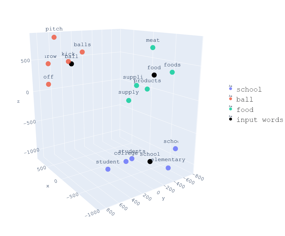
In the following image we can see a 3-dimensional representation of words, and we can see that all words related to school are close together, all words related to food are close together, and all words related to ball are close together.
Having each dimension of the vectors represent a feature of the word allows us to perform operations with words. For example, if we subtract the word man from the word king and add the word woman, we get a word very similar to the word queen. We will verify this with an example later.
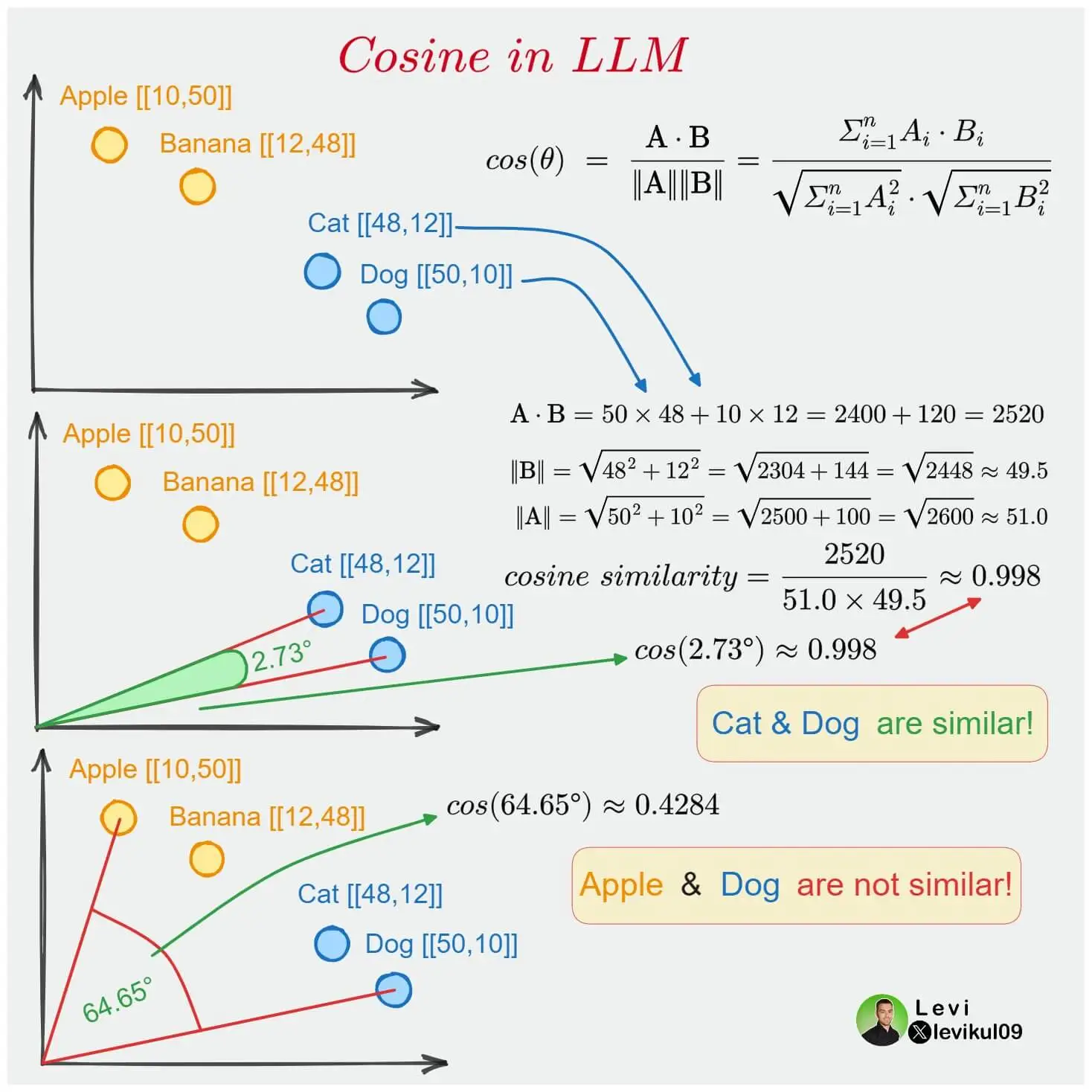
Word Similarity
As each word is represented by an N-dimensional vector, we can calculate the similarity between two words. For this purpose, the cosine similarity function or cosine similarity is used.
If two words are close in the vector space, it means that the angle between their vectors is small, so their cosine is close to 1. If there is a 90-degree angle between the vectors, the cosine is 0, meaning there is no similarity between the words. And if there is a 180-degree angle between the vectors, the cosine is -1, meaning the words are opposites.
Example with OpenAI Embeddings
Now that we know what embeddings are, let's look at some examples with the embeddings provided by the OpenAI API.
To do this, we first need to have the OpenAI package installed.
pip install openaiWe import the necessary libraries
from openai import OpenAIimport torchfrom torch.nn.functional import cosine_similarityCopied
We use an API key from OpenAI. To do this, we go to the OpenAI page and register. Once registered, we navigate to the API Keys section and create a new API Key.
api_key = "Pon aquí tu API key"Copied
We select the embedding model we want to use. In this case, we will use text-embedding-ada-002, which is the one recommended by OpenAI in their embeddings documentation.
model_openai = "text-embedding-ada-002"Copied
We create an API client
client_openai = OpenAI(api_key=api_key, organization=None)Copied
Let's see what the embeddings of the word King look like.
word = "Rey"embedding_openai = torch.Tensor(client_openai.embeddings.create(input=word, model=model_openai).data[0].embedding)embedding_openai.shape, embedding_openaiCopied
(torch.Size([1536]),tensor([-0.0103, -0.0005, -0.0189, ..., -0.0009, -0.0226, 0.0045]))
As we can see, we obtain a vector of 1536 dimensions
Example with HuggingFace embeddings
Since OpenAI's embedding generation is paid, we are going to see how to use HuggingFace embeddings, which are free. To do this, first we need to make sure the sentence-transformers library is installed.
pip install -U sentence-transformersAnd now we start generating the word embeddings.
First we import the library
from sentence_transformers import SentenceTransformerCopied
Now we create an embeddings model from HuggingFace. We use paraphrase-MiniLM-L6-v2 because it is a small and fast model that gives good results, and for our example, it suffices.
model = SentenceTransformer('paraphrase-MiniLM-L6-v2')Copied
And now we can generate the embeddings of the words
sentence = ['Rey']embedding_huggingface = model.encode(sentence)embedding_huggingface.shape, embedding_huggingface[0]Copied
((1, 384),array([ 4.99837071e-01, -7.60397986e-02, 5.47384083e-01, 1.89465046e-01,-3.21713984e-01, -1.01025246e-01, 6.44087136e-01, 4.91398573e-01,3.73571329e-02, -2.77234882e-01, 4.34713453e-01, -1.06284058e+00,2.44114518e-01, 8.98794234e-01, 4.74923879e-01, -7.48904228e-01,2.84665376e-01, -1.75070837e-01, 5.92192829e-01, -1.02512836e-02,9.45721626e-01, 2.43777707e-01, 3.91995460e-01, 3.35530996e-01,-4.58333105e-01, 1.18869759e-01, 5.31717360e-01, -1.21750660e-01,-5.45580745e-01, -7.63889611e-01, -3.19075316e-01, 2.55386919e-01,-4.06407446e-01, -8.99556637e-01, 6.34190366e-02, -2.96231866e-01,-1.22994244e-01, 7.44934231e-02, -4.49327320e-01, -2.71379113e-01,-3.88012260e-01, -2.82730222e-01, 2.50365853e-01, 3.06314558e-01,5.01561277e-02, -5.73592126e-01, -4.93096076e-02, -2.54629493e-01,4.45663840e-01, -1.54654181e-03, 1.85357735e-01, 2.49421135e-01,7.80077875e-01, -2.99735814e-01, 7.34686375e-01, 9.35385004e-02,-8.64403173e-02, 5.90056717e-01, 9.62065995e-01, -3.89911681e-02,4.52635378e-01, 1.10802782e+00, -4.28262979e-01, 8.98583114e-01,-2.79768258e-01, -7.25559890e-01, 4.38431054e-01, 6.08255446e-01,-1.06222546e+00, 1.86217821e-03, 5.23232877e-01, -5.59782684e-01,1.08870542e+00, -1.29855171e-01, -1.34669527e-01, 4.24595959e-02,2.99118191e-01, -2.53481418e-01, -1.82368979e-01, 9.74772453e-01,-7.66527832e-01, 2.02146843e-01, -9.27186012e-01, -3.72025579e-01,2.51360565e-01, 3.66043419e-01, 3.58169287e-01, -5.50914466e-01,3.87659878e-01, 2.67650932e-01, -1.30100116e-01, -9.08647776e-02,2.58671075e-01, -4.44935560e-01, -1.43231079e-01, -2.83272982e-01,7.21463636e-02, 1.98998764e-01, -9.47986841e-02, 1.74529219e+00,1.71559617e-01, 5.96294463e-01, 1.38505893e-02, 3.90956283e-01,3.46427560e-01, 2.63105750e-01, 2.64972121e-01, -2.67196923e-01,7.54366294e-02, 9.39224422e-01, 3.35206270e-01, -1.99105024e-01,-4.06340271e-01, 3.83643419e-01, 4.37904626e-01, 8.92579079e-01,-5.86432815e-01, -2.59302586e-01, -6.39415443e-01, 1.21703267e-01,6.44594133e-01, 2.56335083e-02, 5.53315282e-02, 5.85618019e-01,1.03075497e-01, -4.17360187e-01, 5.00189543e-01, 4.23062295e-01,-7.62073815e-01, -4.36184794e-01, -4.13090199e-01, -2.14746520e-01,3.76077414e-01, -1.51846036e-02, -6.51694953e-01, 2.05930993e-01,-3.73996288e-01, 1.14034235e-01, -7.40544260e-01, 1.98710993e-01,-6.66027904e-01, 3.00016254e-01, -4.03109461e-01, 1.85078502e-01,-3.27183425e-01, 4.19003010e-01, 1.16863050e-01, -4.33366179e-01,3.62291127e-01, 6.25310719e-01, -3.34749371e-01, 3.18448655e-02,-9.09660235e-02, 3.58690947e-01, 1.23402506e-01, -5.08333087e-01,4.18513209e-01, 5.83032072e-01, -8.37822199e-01, -1.52947128e-01,5.07765234e-01, -2.90990144e-01, -2.56464798e-02, 5.69117546e-01,-5.43118417e-01, -3.27799052e-01, -1.70862004e-01, 4.14014012e-01,4.74694878e-01, 5.15708327e-01, 3.21234539e-02, 1.55380607e-01,-3.21141332e-01, -1.72114551e-01, 6.43211603e-01, -3.89207341e-02,-2.29103401e-01, 4.13877398e-01, -9.22305062e-02, -4.54976231e-01,-1.50242126e+00, -2.81573564e-01, 1.70057654e-01, 4.53076512e-01,-4.25060362e-01, -1.33391351e-01, 5.40394569e-03, 3.71117502e-01,-4.29107875e-01, 1.35897202e-02, 2.44936779e-01, 1.04574718e-01,-3.65612388e-01, 4.33572650e-01, -4.09719855e-01, -2.95067448e-02,1.26362443e-02, -7.43583977e-01, -7.35885441e-01, -1.35508239e-01,-2.12558493e-01, -5.46157181e-01, 7.55161867e-02, -3.57991695e-01,-1.20607555e-01, 5.53125329e-02, -3.23110700e-01, 4.88573104e-01,-1.07487953e+00, 1.72190830e-01, 8.48749802e-02, 5.73584400e-02,3.06147277e-01, 3.26699704e-01, 5.09487510e-01, -2.60940105e-01,-2.85459042e-01, 3.15197736e-01, -8.84049162e-02, -2.14854136e-01,4.04228538e-01, -3.53874594e-01, 3.30587216e-02, -2.04278827e-01,4.45132256e-01, -4.05272096e-01, 9.07981098e-01, -1.70708492e-01,3.62848401e-01, -3.17223936e-01, 1.53909430e-01, 7.24429131e-01,2.27339968e-01, -1.16330147e+00, -9.58504915e-01, 4.87008452e-01,-2.30886355e-01, -1.40117988e-01, 7.84571916e-02, -2.93157458e-01,1.00778294e+00, 1.34625390e-01, -4.66320179e-02, 6.51122704e-02,-1.50451362e-02, -2.15500608e-01, -2.42915586e-01, -3.21900517e-01,-2.94186682e-01, 4.71027017e-01, 1.56058431e-01, 1.30854800e-01,-2.84257025e-01, -1.44421116e-01, -7.09840000e-01, -1.80235609e-01,-8.30230191e-02, 9.08326149e-01, -8.22497830e-02, 1.46948382e-01,-1.41326815e-01, 3.81170362e-01, -6.37023628e-01, 1.70148894e-01,-1.00046806e-01, 5.70729785e-02, -1.09820545e+00, -1.03613675e-01,-6.21219516e-01, 4.55532551e-01, 1.86942443e-01, -2.04409719e-01,7.81394243e-01, -7.88963258e-01, 2.19068691e-01, -3.62780124e-01,-3.41522694e-01, -1.73794985e-01, -4.00943428e-01, 5.01900315e-01,4.53949839e-01, 1.03774257e-01, -1.66873619e-01, -4.63893116e-02,-1.78147718e-01, 4.85655308e-01, -3.02978605e-02, -5.67060888e-01,-4.68107373e-01, -6.57559693e-01, -5.02855539e-01, -1.94635347e-01,-9.58659649e-01, -4.97986436e-01, 1.33874401e-01, 3.09395105e-01,-4.52993363e-01, 7.43827343e-01, -1.87271550e-01, -6.11483693e-01,-1.08927953e+00, -2.30332208e-03, 2.11169615e-01, -3.46892715e-01,-3.32458824e-01, 2.07640216e-01, -4.10387546e-01, 3.12181324e-01,3.69687408e-01, 8.62928331e-01, 2.40735337e-01, -3.65841389e-02,6.84210837e-01, 3.45884450e-02, 5.63964128e-01, 2.39361122e-01,3.10872793e-01, -6.34638309e-01, -9.07931089e-01, -6.35836497e-02,2.20288679e-01, 2.59186536e-01, -4.45540816e-01, 6.33085072e-01,-1.97424471e-01, 7.51152515e-01, -2.68558711e-01, -4.39288855e-01,4.13556695e-01, -1.89288303e-01, 5.81856608e-01, 4.75860722e-02,1.60344616e-01, -2.96180040e-01, 2.91323394e-01, 1.34404674e-01,-1.22037649e-01, 4.19363379e-02, -3.87936801e-01, -9.25336123e-01,-5.28307915e-01, -1.74257740e-01, -1.52818128e-01, 4.31716293e-02,-2.12064430e-01, 2.98252910e-01, 9.86064151e-02, 3.84781063e-02,6.68018535e-02, -2.29525566e-01, -8.20755959e-03, 5.17108142e-01,-6.66776478e-01, -1.38897672e-01, 4.68370765e-01, -2.14766636e-01,2.43549764e-01, 2.25854263e-01, -1.92763060e-02, 2.78505355e-01,3.39088053e-01, -9.69757214e-02, -2.71263003e-01, 1.05703615e-01,1.14365645e-01, 4.16649908e-01, 4.18699026e-01, -1.76222697e-01,-2.08620593e-01, -5.79392374e-01, -1.68948188e-01, -1.77841976e-01,5.69338985e-02, 2.12916449e-01, 4.24367547e-01, -7.13860095e-02,8.28932896e-02, -2.40542665e-01, -5.94049037e-01, 4.09415931e-01,1.01326215e+00, -5.71239054e-01, 4.35258061e-01, -3.64619821e-01],dtype=float32))
As we can see, we obtain a vector of 384 dimensions. In this case, a vector of this dimension is obtained because the model paraphrase-MiniLM-L6-v2 has been used. If we use another model, we will obtain vectors of different dimensions.
Operations with words
Let's get the embeddings of the words king, man, woman, and queen.
embedding_openai_rey = torch.Tensor(client_openai.embeddings.create(input="rey", model=model_openai).data[0].embedding)embedding_openai_hombre = torch.Tensor(client_openai.embeddings.create(input="hombre", model=model_openai).data[0].embedding)embedding_openai_mujer = torch.Tensor(client_openai.embeddings.create(input="mujer", model=model_openai).data[0].embedding)embedding_openai_reina = torch.Tensor(client_openai.embeddings.create(input="reina", model=model_openai).data[0].embedding)Copied
embedding_openai_reina.shape, embedding_openai_reinaCopied
(torch.Size([1536]),tensor([-0.0110, -0.0084, -0.0115, ..., 0.0082, -0.0096, -0.0024]))
Let's obtain the resulting embedding by subtracting the man embedding from the king embedding and adding the woman embedding.
embedding_openai = embedding_openai_rey - embedding_openai_hombre + embedding_openai_mujerCopied
embedding_openai.shape, embedding_openaiCopied
(torch.Size([1536]),tensor([-0.0226, -0.0323, 0.0017, ..., 0.0014, -0.0290, -0.0188]))
Finally, we compare the obtained result with the embedding of queen. For this, we use the cosine_similarity function provided by the pytorch library.
similarity_openai = cosine_similarity(embedding_openai.unsqueeze(0), embedding_openai_reina.unsqueeze(0)).item()print(f"similarity_openai: {similarity_openai}")Copied
similarity_openai: 0.7564167976379395
As we can see, it is a value very close to 1, so we can say that the result obtained is very similar to the embedding of queen
If we use English words, we get a result closer to 1
embedding_openai_rey = torch.Tensor(client_openai.embeddings.create(input="king", model=model_openai).data[0].embedding)embedding_openai_hombre = torch.Tensor(client_openai.embeddings.create(input="man", model=model_openai).data[0].embedding)embedding_openai_mujer = torch.Tensor(client_openai.embeddings.create(input="woman", model=model_openai).data[0].embedding)embedding_openai_reina = torch.Tensor(client_openai.embeddings.create(input="queen", model=model_openai).data[0].embedding)Copied
embedding_openai = embedding_openai_rey - embedding_openai_hombre + embedding_openai_mujerCopied
similarity_openai = cosine_similarity(embedding_openai.unsqueeze(0), embedding_openai_reina.unsqueeze(0))print(f"similarity_openai: {similarity_openai}")Copied
similarity_openai: tensor([0.8849])
This is normal, since the OpenAI model has been trained with more English texts than Spanish.
Types of Word Embeddings
There are several types of word embeddings, and each of them has its advantages and disadvantages. Let's look at the most important ones.
- Word2Vec
- GloVe
- FastText
- BERT
- GPT-2
Word2Vec
Word2Vec is an algorithm used to create word embeddings. This algorithm was created by Google in 2013, and it is one of the most widely used algorithms for creating word embeddings.
It has two variants, CBOW and Skip-gram. CBOW is faster to train, while Skip-gram is more accurate. Let's see how each of them works.
CBOW
CBOW or Continuous Bag of Words is an algorithm used to predict a word based on the words surrounding it. For example, if we have the sentence The cat is an animal, the algorithm will try to predict the word cat based on the surrounding words, in this case The, is, an, and animal.
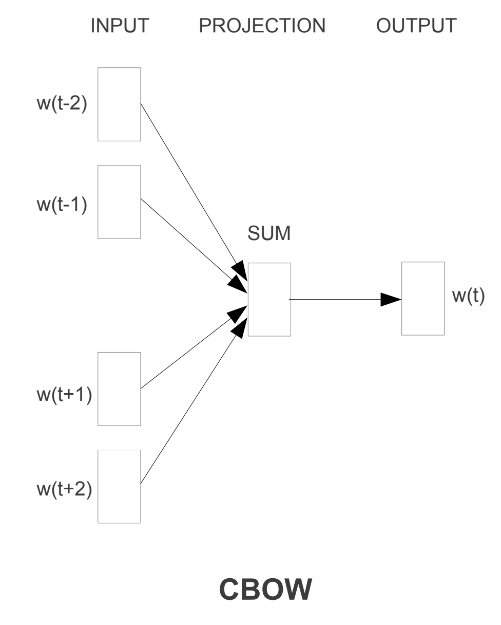
In this architecture, the model predicts which word is most likely in the given context. Therefore, words that have the same probability of appearing are considered similar and thus move closer together in the dimensional space.
Let's assume that in a sentence we replace barco with bote, then the model predicts the probability for both and if it turns out to be similar, we can consider the words to be similar.
Skip-gram
Skip-gram or Skip-gram with Negative Sampling is an algorithm used to predict the words surrounding a given word. For example, if we have the sentence The cat is an animal, the algorithm will try to predict the words The, is, an, and animal based on the word cat.
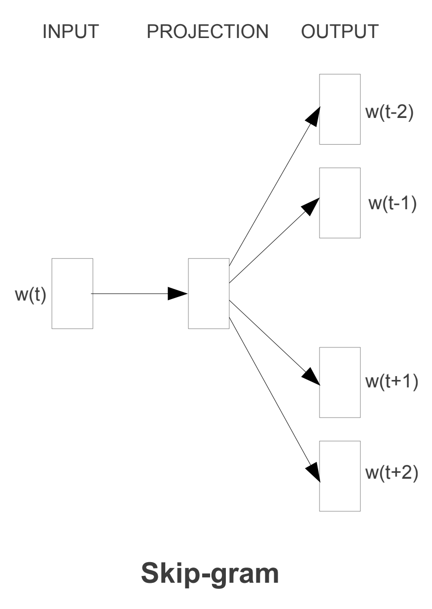
This architecture is similar to that of CBOW, but instead the model works in reverse. The model predicts the context using the given word. Therefore, words that have the same context are considered similar and thus move closer together in the dimensional space.
GloVe
GloVe or Global Vectors for Word Representation is an algorithm used to create word embeddings. This algorithm was developed by Stanford University in 2014.
Word2Vec ignores the fact that some context words occur more frequently than others and also only takes into account the local context, and therefore, does not capture the global context.
This algorithm uses a co-occurrence matrix to create the word embeddings. This co-occurrence matrix is a matrix that contains the number of times each word appears alongside each of the other words in the vocabulary.
FastText
FastText is an algorithm used to create word embeddings. This algorithm was created by Facebook in 2016.
One of the main disadvantages of Word2Vec and GloVe is that they cannot encode unknown words or out-of-vocabulary words.
So, to deal with this problem, Facebook proposed a model FastText. It is an extension of Word2Vec and follows the same Skip-gram and CBOW models. However, unlike Word2Vec which feeds whole words into the neural network, FastText first splits the words into several subwords (or n-grams) and then feeds them into the neural network.
For example, if the value of n is 3 and the word is manzana then its tri-gram will be [<ma, man, anz, nza, zan, ana, na>] and its word embedding will be the sum of the vector representation of these tri-grams. Here, the hyperparameters min_n and max_n are considered as 3 and the characters < and > represent the beginning and end of the word.
Therefore, using this methodology, unknown words can be represented in vector form, as they have a high probability that their n-grams are also present in other words.
This algorithm is an improvement over Word2Vec, as it not only takes into account the words surrounding a word, but also considers the n-grams of the word. For example, if we have the word gato, it also takes into account the n-grams of the word, in this case ga, at, and to, for n = 2.
Limitations of Word Embeddings
Word embedding techniques have yielded decent results, but the problem is that the approach is not accurate enough. They do not take into account the order in which words appear, leading to a loss of syntactic and semantic understanding of the sentence.
For example, You go there to teach, not to play and You go there to play, not to teach Both sentences will have the same representation in the vector space, but they do not mean the same thing.
Moreover, the word embedding model cannot provide satisfactory results on a large amount of text data, as the same word can have a different meaning in a different sentence depending on the context of the sentence.
For example, I'm going to sit on the bench and I'm going to do some errands at the bank. In both sentences, the word bank has different meanings.
Therefore, we require a type of representation that can retain the contextual meaning of the word present in a sentence.
Sentence embeddings
The sentence embedding is similar to the word embedding, but instead of words, it encodes the entire sentence into the vector representation.
A simple way to obtain sentence embeddings is by averaging the word embeddings of all the words present in the sentence. But they are not accurate enough.
Some of the most advanced models for sentence embedding are ELMo, InferSent, and Sentence-BERT
ELMo
ELMo or Embeddings from Language Models is a sentence embedding model created by the Allen University in 2018. It uses a deep bidirectional LSTM network to produce vector representations. ELMo can represent unknown words or out-of-vocabulary words in vector form since it is character-based.
InferSent
InferSent is a sentence embedding model created by Facebook in 2017. It uses a deep bidirectional LSTM network to produce a vector representation. InferSent can represent unknown or out-of-vocabulary words in vector form, as it is character-based. Sentences are encoded into a 4096-dimensional vector representation.
The model training is performed on the Stanford Natural Language Inference (SNLI) dataset. This dataset is labeled and written by humans for around 500K sentence pairs.
Sentence-BERT
Sentence-BERT is a sentence embedding model created by the University of London in 2019. It uses a deep bidirectional LSTM network to produce vector representations. Sentence-BERT can represent unknown or out-of-vocabulary words in vector form since it is character-based. Sentences are encoded into a 768-dimensional vector representation.
The state-of-the-art NLP model BERT excels in Semantic Textual Similarity tasks, but the issue is that it would take a long time for a huge corpus (65 hours for 10,000 sentences), as it requires both sentences to be fed into the network, which increases the computation by an enormous factor.
Therefore, Sentence-BERT is a modification of the BERT model.
Training a word2vec model with gensim
To download the dataset we are going to use, you need to install the dataset library from huggingface:
pip install datasetsTo train the embeddings model, we will use the gensim library. To install it with Conda, we use
conda install -c conda-forge gensimAnd to install it with pip we use
pip install gensimTo clean the dataset we have downloaded, we are going to use regular expressions, which is usually already installed in Python, and nltk, which is a natural language processing library. To install it with Conda, we use
conda install -c anaconda nltkAnd to install it with pip we use
pip install nltkNow that we have everything installed, we can import the libraries we are going to use:
from gensim.models import Word2Vecfrom gensim.parsing.preprocessing import strip_punctuation, strip_numeric, strip_shortimport refrom nltk.corpus import stopwordsfrom nltk.tokenize import word_tokenizeCopied
Download the dataset
We are going to download a dataset of texts from the Spanish Wikipedia. To do this, we run the following:
from datasets import load_datasetdataset_corpus = load_dataset('large_spanish_corpus', name='all_wikis')Copied
Let's see how it is
dataset_corpusCopied
DatasetDict({train: Dataset({features: ['text'],num_rows: 28109484})})
As we can see, the dataset has more than 28 million texts. Let's take a look at some of them:
dataset_corpus['train']['text'][0:10]Copied
['¡Bienvenidos!','Ir a los contenidos»','= Contenidos =','','Portada','Tercera Lengua más hablada en el mundo.','La segunda en número de habitantes en el mundo occidental.','La de mayor proyección y crecimiento día a día.','El español es, hoy en día, nombrado en cada vez más contextos, tomando realce internacional como lengua de cultura y civilización siempre de mayor envergadura.','Ejemplo de ello es que la comunidad minoritaria más hablada en los Estados Unidos es precisamente la que habla idioma español.']
As there are many examples, we are going to create a subset of 10 million examples to be able to work faster:
subset = dataset_corpus['train'].select(range(10000000))Copied
Cleaning the dataset
Now we download the stopwords from nltk, which are words that do not provide information and that we are going to remove from the texts.
import nltknltk.download('stopwords')Copied
[nltk_data] Downloading package stopwords to[nltk_data] /home/wallabot/nltk_data...[nltk_data] Package stopwords is already up-to-date!
True
Now we are going to download the punkt from nltk, which is a tokenizer that will allow us to split the texts into sentences.
nltk.download('punkt')Copied
[nltk_data] Downloading package punkt to /home/wallabot/nltk_data...[nltk_data] Package punkt is already up-to-date!
True
We create a function to clean the data. This function will:
- convert the text to lowercase
- Remove the URLs
- Remove mentions of social media such as
@twitterand#hashtag - Remove punctuation marks
- Remove the numbers
- Remove short words
- Remove the stop words
Since we are using a huggingface dataset, the texts are in dict format, so we return a dictionary.
def clean_text(sentence_batch):# extrae el texto de la entradatext_list = sentence_batch['text']cleaned_text_list = []for text in text_list:# Convierte el texto a minúsculastext = text.lower()# Elimina URLstext = re.sub(r'httpS+|wwwS+|httpsS+', '', text, flags=re.MULTILINE)# Elimina las menciones @ y '#' de las redes socialestext = re.sub(r'@w+|#w+', '', text)# Elimina los caracteres de puntuacióntext = strip_punctuation(text)# Elimina los númerostext = strip_numeric(text)# Elimina las palabras cortastext = strip_short(text,minsize=2)# Elimina las palabras comunes (stop words)stop_words = set(stopwords.words('spanish'))word_tokens = word_tokenize(text)filtered_text = [word for word in word_tokens if word not in stop_words]cleaned_text_list.append(filtered_text)# Devuelve el texto limpioreturn {'text': cleaned_text_list}Copied
We apply the function to the data
sentences_corpus = subset.map(clean_text, batched=True)Copied
Map: 0%| | 0/10000000 [00:00<?, ? examples/s]
Let's save the filtered dataset to a file so we don't have to run the cleaning process again.
sentences_corpus.save_to_disk("sentences_corpus")Copied
Saving the dataset (0/4 shards): 0%| | 0/15000000 [00:00<?, ? examples/s]
To load it we can do
from datasets import load_from_disksentences_corpus = load_from_disk('sentences_corpus')Copied
Now we will have a list of lists, where each list is a tokenized sentence and without stopwords. That is, we have a list of sentences, and each sentence is a list of words. Let's see how it looks:
for i in range(10):print(f'La frase "{subset["text"][i]}" se convierte en la lista de palabras "{sentences_corpus["text"][i]}"')Copied
La frase "¡Bienvenidos!" se convierte en la lista de palabras "['¡bienvenidos']"La frase "Ir a los contenidos»" se convierte en la lista de palabras "['ir', 'contenidos', '»']"La frase "= Contenidos =" se convierte en la lista de palabras "['contenidos']"La frase "" se convierte en la lista de palabras "[]"La frase "Portada" se convierte en la lista de palabras "['portada']"La frase "Tercera Lengua más hablada en el mundo." se convierte en la lista de palabras "['tercera', 'lengua', 'hablada', 'mundo']"La frase "La segunda en número de habitantes en el mundo occidental." se convierte en la lista de palabras "['segunda', 'número', 'habitantes', 'mundo', 'occidental']"La frase "La de mayor proyección y crecimiento día a día." se convierte en la lista de palabras "['mayor', 'proyección', 'crecimiento', 'día', 'día']"La frase "El español es, hoy en día, nombrado en cada vez más contextos, tomando realce internacional como lengua de cultura y civilización siempre de mayor envergadura." se convierte en la lista de palabras "['español', 'hoy', 'día', 'nombrado', 'cada', 'vez', 'contextos', 'tomando', 'realce', 'internacional', 'lengua', 'cultura', 'civilización', 'siempre', 'mayor', 'envergadura']"La frase "Ejemplo de ello es que la comunidad minoritaria más hablada en los Estados Unidos es precisamente la que habla idioma español." se convierte en la lista de palabras "['ejemplo', 'ello', 'comunidad', 'minoritaria', 'hablada', 'unidos', 'precisamente', 'habla', 'idioma', 'español']"
Training the word2vec model
We are going to train an embedding model that will convert words into vectors. For this, we will use the gensim library and its Word2Vec model.
dataset = sentences_corpus['text']dim_embedding = 100window_size = 5 # 5 palabras a la izquierda y 5 palabras a la derechamin_count = 5 # Ignora las palabras con frecuencia menor a 5workers = 4 # Número de hilos de ejecuciónsg = 1 # 0 para CBOW, 1 para Skip-grammodel = Word2Vec(dataset, vector_size=dim_embedding, window=window_size, min_count=min_count, workers=workers, sg=sg)Copied
This model has been trained on the CPU, since gensim does not have an option to perform training on the GPU and even so, it took X minutes to train the model on my computer. Although the embedding dimension we chose is only 100 (as opposed to the size of OpenAI's embeddings which is 1536), this is not too long a time, given that the dataset has 10 million sentences.
Large language models are trained with datasets consisting of billions of sentences, so it's normal for training an embeddings model with a dataset of 10 million sentences to take several minutes.
Once the model is trained, we save it to a file so that we can use it in the future.
model.save('word2vec.model')Copied
If we wanted to load it in the future, we could do so with
model = Word2Vec.load('word2vec.model')Copied
Evaluation of the word2vec model
Let's look at the most similar words for some words
model.wv.most_similar('perro', topn=10)Copied
[('gato', 0.7948548197746277),('perros', 0.77247554063797),('cachorro', 0.7638891339302063),('hámster', 0.7540281414985657),('caniche', 0.7514827251434326),('bobtail', 0.7492328882217407),('mastín', 0.7491254210472107),('lobo', 0.7312178611755371),('semental', 0.7292628288269043),('sabueso', 0.7290207147598267)]
model.wv.most_similar('gato', topn=10)Copied
[('conejo', 0.8148329854011536),('zorro', 0.8109457492828369),('perro', 0.7948548793792725),('lobo', 0.7878773808479309),('ardilla', 0.7860757112503052),('mapache', 0.7817519307136536),('huiña', 0.766639232635498),('oso', 0.7656188011169434),('mono', 0.7633568644523621),('camaleón', 0.7623056769371033)]
Now let's look at the example where we check the similarity of the word queen with the result of subtracting the word man from the word king and adding the word woman
embedding_hombre = model.wv['hombre']embedding_mujer = model.wv['mujer']embedding_rey = model.wv['rey']embedding_reina = model.wv['reina']Copied
embedding = embedding_rey - embedding_hombre + embedding_mujerCopied
from torch.nn.functional import cosine_similarityembedding = torch.tensor(embedding).unsqueeze(0)embedding_reina = torch.tensor(embedding_reina).unsqueeze(0)similarity = cosine_similarity(embedding, embedding_reina, dim=1)similarityCopied
tensor([0.8156])
As we can see, there is quite a bit of similarity
Visualization of the embeddings
Let's visualize the embeddings. First, we'll obtain the vectors and words from the model.
embeddings = model.wv.vectorswords = list(model.wv.index_to_key)Copied
Since the dimension of the embeddings is 100, to be able to visualize them in 2 or 3 dimensions we have to reduce the dimension. For this, we will use PCA (faster) or TSNE (more accurate) from sklearn
from sklearn.decomposition import PCAdimmesions = 2pca = PCA(n_components=dimmesions)reduced_embeddings_PCA = pca.fit_transform(embeddings)Copied
from sklearn.manifold import TSNEdimmesions = 2tsne = TSNE(n_components=dimmesions, verbose=1, perplexity=40, n_iter=300)reduced_embeddings_tsne = tsne.fit_transform(embeddings)Copied
[t-SNE] Computing 121 nearest neighbors...[t-SNE] Indexed 493923 samples in 0.013s...[t-SNE] Computed neighbors for 493923 samples in 377.143s...[t-SNE] Computed conditional probabilities for sample 1000 / 493923[t-SNE] Computed conditional probabilities for sample 2000 / 493923[t-SNE] Computed conditional probabilities for sample 3000 / 493923[t-SNE] Computed conditional probabilities for sample 4000 / 493923[t-SNE] Computed conditional probabilities for sample 5000 / 493923[t-SNE] Computed conditional probabilities for sample 6000 / 493923[t-SNE] Computed conditional probabilities for sample 7000 / 493923[t-SNE] Computed conditional probabilities for sample 8000 / 493923[t-SNE] Computed conditional probabilities for sample 9000 / 493923[t-SNE] Computed conditional probabilities for sample 10000 / 493923[t-SNE] Computed conditional probabilities for sample 11000 / 493923[t-SNE] Computed conditional probabilities for sample 12000 / 493923[t-SNE] Computed conditional probabilities for sample 13000 / 493923[t-SNE] Computed conditional probabilities for sample 14000 / 493923[t-SNE] Computed conditional probabilities for sample 15000 / 493923[t-SNE] Computed conditional probabilities for sample 16000 / 493923[t-SNE] Computed conditional probabilities for sample 17000 / 493923[t-SNE] Computed conditional probabilities for sample 18000 / 493923[t-SNE] Computed conditional probabilities for sample 19000 / 493923[t-SNE] Computed conditional probabilities for sample 20000 / 493923[t-SNE] Computed conditional probabilities for sample 21000 / 493923[t-SNE] Computed conditional probabilities for sample 22000 / 493923...[t-SNE] Computed conditional probabilities for sample 493923 / 493923[t-SNE] Mean sigma: 0.275311[t-SNE] KL divergence after 250 iterations with early exaggeration: 117.413788[t-SNE] KL divergence after 300 iterations: 5.774648
Now we visualize them in 2 dimensions with matplotlib. We are going to visualize the dimensionality reduction we have done with PCA and TSNE.
import matplotlib.pyplot as pltplt.figure(figsize=(10, 10))for i, word in enumerate(words[:200]): # Limitar a las primeras 200 palabrasplt.scatter(reduced_embeddings_PCA[i, 0], reduced_embeddings_PCA[i, 1])plt.annotate(word, xy=(reduced_embeddings_PCA[i, 0], reduced_embeddings_PCA[i, 1]), xytext=(5, 2), textcoords='offset points', ha='right', va='bottom')plt.title('Embeddings (PCA)')plt.show()Copied
<Figure size 1000x1000 with 1 Axes>
plt.figure(figsize=(10, 10))for i, word in enumerate(words[:200]): # Limitar a las primeras 200 palabrasplt.scatter(reduced_embeddings_tsne[i, 0], reduced_embeddings_tsne[i, 1])plt.annotate(word, xy=(reduced_embeddings_tsne[i, 0], reduced_embeddings_tsne[i, 1]), xytext=(5, 2),textcoords='offset points', ha='right', va='bottom')plt.show()Copied
<Figure size 1000x1000 with 1 Axes>
Using Pretrained Models with HuggingFace
To use pre-trained embedding models, we will use the transformers library from huggingface. To install it with Conda, we use
conda install -c conda-forge transformersAnd to install it with pip we use
pip install transformersWith the feature-extraction task from huggingface, we can use pretrained models to obtain word embeddings. To do this, we first import the necessary library.
from transformers import pipelineCopied
We are going to obtain the embeddings from BERT
checkpoint = "bert-base-uncased"feature_extractor = pipeline("feature-extraction",framework="pt",model=checkpoint)Copied
Let's look at the embeddings of the word king
embedding = feature_extractor("rey", return_tensors="pt").squeeze(0)embedding.shapeCopied
torch.Size([3, 768])
As we can see, we obtain a vector of 768 dimensions, that is, the embeddings of BERT have 768 dimensions. On the other hand, we see that it has 3 embedding vectors, this is because BERT adds a token at the beginning and another at the end of the sentence, so we are only interested in the middle vector.
Let's redo the example where we check the similarity of the word queen with the result of subtracting the word man from the word king and adding the word woman
embedding_hombre = feature_extractor("man", return_tensors="pt").squeeze(0)[1]embedding_mujer = feature_extractor("woman", return_tensors="pt").squeeze(0)[1]embedding_rey = feature_extractor("king", return_tensors="pt").squeeze(0)[1]embedding_reina = feature_extractor("queen", return_tensors="pt").squeeze(0)[1]Copied
embedding = embedding_rey - embedding_hombre + embedding_mujerCopied
Let's see the similarity
import torchfrom torch.nn.functional import cosine_similarityembedding = torch.tensor(embedding).unsqueeze(0)embedding_reina = torch.tensor(embedding_reina).unsqueeze(0)similarity = cosine_similarity(embedding, embedding_reina, dim=1)similarity.item()Copied
/tmp/ipykernel_33343/4248442045.py:4: UserWarning: To copy construct from a tensor, it is recommended to use sourceTensor.clone().detach() or sourceTensor.clone().detach().requires_grad_(True), rather than torch.tensor(sourceTensor).embedding = torch.tensor(embedding).unsqueeze(0)/tmp/ipykernel_33343/4248442045.py:5: UserWarning: To copy construct from a tensor, it is recommended to use sourceTensor.clone().detach() or sourceTensor.clone().detach().requires_grad_(True), rather than torch.tensor(sourceTensor).embedding_reina = torch.tensor(embedding_reina).unsqueeze(0)
0.742547333240509
Using the embeddings of BERT also yields a result very close to 1