How Neural Networks Work: Linear Regression and Gradient Descent Step by Step

04 of october of 2025

Disclaimer: This post has been translated to English using a machine translation model. Please, let me know if you find any mistakes.

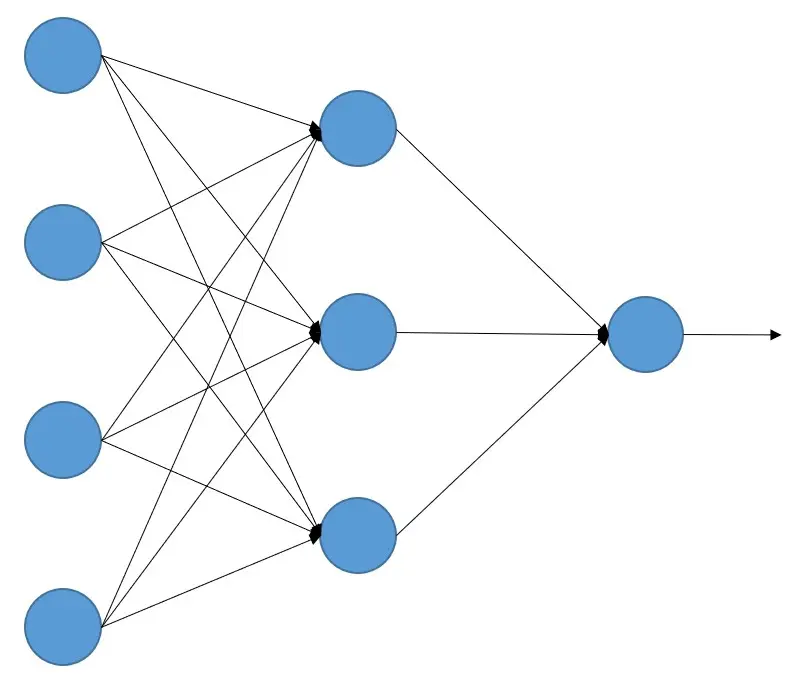
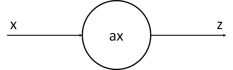
As we have said, a neuron is a processing unit, it receives some signals, performs some calculations, and produces another signal.

So let's look at the simplest example, the case in which a signal is received and another is output, and we'll see it using linear regression.

!neural network regression

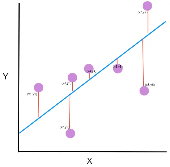
Let's suppose we have made some measurements and obtained the following points

	
		import numpy as np
 
x = np.array( [ 0. , 0.34482759, 0.68965517, 1.03448276, 1.37931034,
        1.72413793, 2.06896552, 2.4137931 , 2.75862069, 3.10344828,
        3.44827586, 3.79310345, 4.13793103, 4.48275862, 4.82758621,
        5.17241379, 5.51724138, 5.86206897, 6.20689655, 6.55172414,
        6.89655172, 7.24137931, 7.5862069 , 7.93103448, 8.27586207,
        8.62068966, 8.96551724, 9.31034483, 9.65517241, 10. ])
 
z = np.array( [-0.16281253, 1.88707606, 0.39649312, 0.03857752, 4.0148778 ,
        0.58866234, 3.35711859, 1.94314906, 6.96106424, 5.89792585,
        8.47226615, 3.67698542, 12.05958678, 9.85234481, 9.82181679,
        6.07652248, 14.17536744, 12.67825433, 12.97499286, 11.76098542,
       12.7843083 , 16.42241036, 13.67913705, 15.55066478, 17.45979602,
       16.41982806, 17.01977617, 20.28151197, 19.38148414, 19.41029831])
	
	
		
	
	Copied

	
		import matplotlib.pyplot as plt
 
plt.scatter(x, z)
plt.xlabel('X')
plt.ylabel('Z  ', rotation=0)
plt.show()
	
	
		
	
	Copied

	
		&lt;Figure size 640x480 with 1 Axes&gt;

As we can see, this can be likened to a linear regression. That is, we can assume that the neuron receives x, multiplies it by a number, and produces z.

From here on, we are going to show how neural networks work, but starting with a simple example of just one neuron. Then we’ll progressively present more complex examples until we explain the general functioning of neural networks. But if you understand what is going to happen next, you will understand neural networks.

Our neuron has the parameter a, which is the one we want to change so that the line it generates resembles the points as closely as possible. The learning process of our neuron will consist of determining the best possible value of a through a series of calculations.

Random Initialization of the Parameter

This example is simple, but when we have complex neural networks and we do not know what values their parameters should have, what is done is to initialize them randomly.

	
		import random
 
random.seed(45) # Esto es una semilla, cuando se generan números aleatorios, 
                # pero queremos que siempre se genere el mismo se suele fijar
                # un número llamado semilla. Esto hace que siempre a sea el mismo
 
a = random.random()
a
	
	
		
	
	Copied

	
		0.2718754143840908

The value of a is 0.271875, let's see what line would result if we stopped now

	
		z_p = a*x
 
plt.scatter(x, z)
plt.plot(x, z_p, 'k')
plt.xlabel('X')
plt.ylabel('Z  ', rotation=0)
plt.show()
	
	
		
	
	Copied

	
		&lt;Figure size 640x480 with 1 Axes&gt;

As we can see, it doesn't look alike at all, so we will have to make our neuron *learn*

Calculation of error or loss

To find the best possible value for a, we want to find a value that makes the outputs predicted by our neuron have the smallest possible error compared to the actual values of z.

In this type of problems, the mean squared error (MSE) is usually used. There are many more error functions, but for now they are not relevant, so stick with this one and we will learn more functions later on.

In the literature, this error is commonly referred to as the loss function, so from now on we will call it that.

The mean squared error (MSE) measures the distance between the points predicted by our neuron and the actual values of z, hence the word *error* in its name.

$(z p - z)$

However, sometimes that distance will be positive and sometimes negative, depending on whether the predicted value from our neuron or the value of z is taken first, so that distance is squared, hence the word *quadratic* in the name.

$(z p -z) 2$

Lastly, all the squared distances are added together and divided by the number of samples—in other words, calculating an average as usual, hence the word *mean* in the name.

$loss = ∑i=1N ≤ft(zp-z\right)2N$

We already have a way to calculate the MSE (mean squared error).

In our case, our loss is

	
		def loss(z, z_p):
    n = len(z)
    loss = np.sum((z_p-z) ** 2) / n
    return loss
	
	
		
	
	Copied

	
		error = loss(z, z_p)
error
	
	
		
	
	Copied

	
		103.72263739946467

Although this does not tell us much, we must remember that we are looking for the minimum of the error function, so we should look for a value close to 0.

Let's see how the loss function changes depending on the value of ```a

```

	
		posibles_a = np.linspace(0, 4, 30)
perdidas = np.empty_like(posibles_a)
 
for i in range (30):
    z_p = posibles_a[i]*x
    perdidas[i] = loss(z, z_p)
 
plt.plot(posibles_a, perdidas)
plt.xlabel('a')
plt.ylabel('loss  ', rotation=0)
plt.show()
	
	
		
	
	Copied

	
		&lt;Figure size 640x480 with 1 Axes&gt;

We can see that the error or loss is smaller when a is around 2. You might think, that's it, problem solved, and that's true. But as I told you, we were going to start with the simplest problem, so by looking at a graph we can solve it.

If the problem had 2 parameters, we could look at a 3-dimensional graph to search for the minimum.

But as soon as our problem has more than 2 parameters, we can no longer look for the minimum error using a graph. Not to mention that neural networks have millions of parameters; for example, the resnet18 neural network (which we will study later) is a small network and has around 11 million parameters. It is impossible to look for the minimum error there manually. So, we need an automatic method using calculations.

Gradient Descent

As we have said, we need to find the value of a that makes the loss function minimal and, at the same time, do so using an algorithm.

One of the peculiarities of a minimum of a function is that its gradient or derivative is 0.

If you don't know what the derivative or gradient is, the derivative of a function at a point represents the slope of the tangent line to the function at that point.

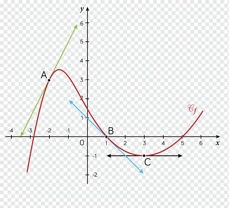
For example, in this image, the derivative of A, B, and C are the green, blue, and black lines, respectively.

The derivative measures the slope of a function; the steeper the function is at a point, the more perpendicular to the *x-axis* the derivative will be at that point, and the less steep the function is at a point, the more parallel to the *x-axis* the derivative will be at that point.

How is the gradient of the loss function with respect to a calculated? We previously defined the loss function as.

$loss = ∑i=1N ≤ft(zp-z\right)2N$

Well, if we differentiate it with respect to a we get

$\partial loss\partial a = \partial ≤ft(∑i=1N ≤ft(zp-z\right)2N\right)\partial a =\partial ≤ft(∑i=1N ≤ft(ax-z\right)2N\right)\partial a = 2N∑i=1N {≤ft(ax-z\right) x} = 2N∑i=1N {≤ft(zp-z\right) x}$

If we look again at the graph of the loss function with respect to the value of a, the steeper the function, that is, the greater the derivative, the further we are from the minimum. And the smaller the derivative, the lesser the slope, the closer we are to the minimum.

	
		def gradiente (a, x, z):
    # Función que calcula el valor de una derivada en un punto
    n = len(z)
    return 2*np.sum((a*x - z)*x)/n
	
	
		
	
	Copied

	
		def gradiente_linea (i, a=None, error=None, gradiente=None):
    # Función que devuleve los puntos de la linea que supone la derivada de una 
    # función en un punto dado
    if a is None:
        x1 = posibles_a[i]-0.7
        x2 = posibles_a[i]
        x3 = posibles_a[i]+0.7
 
        b = perdidas[i] - gradientes[i]*posibles_a[i]
 
        z1 = gradientes[i]*x1 + b
        z2 = perdidas[i]
        z3 = gradientes[i]*x3 + b
    else:
        x1 = a-0.7
        x2 = a
        x3 = a+0.7
 
        b = error - gradiente*a
 
        z1 = gradiente*x1 + b
        z2 = error
        z3 = gradiente*x3 + b
 
    x_linea = np.array([x1, x2, x3])
    z_linea = np.array([z1, z2, z3])
 
    return x_linea, z_linea
	
	
		
	
	Copied

	
		posibles_a = np.linspace(0, 4, 30)
perdidas = np.empty_like(posibles_a)
gradientes = np.empty_like(posibles_a)
 
for i in range (30):
    z_p = posibles_a[i]*x
    perdidas[i] = loss(z, z_p)
    gradientes[i] = gradiente(posibles_a[i], x, z) # Estos son los valores de las derivadas en cada valor de a
                                                    # es decir, nos da el valor de la pendiente de la recta tangente
                                                    # a la curva
 
# Se calcula la linea del gradiente en el inicio
i_inicio = 3
x_inicio, z_inicio = gradiente_linea(i_inicio)
 
# Se calcula la linea del gradiente en la base
i_base = 14
x_base, z_base = gradiente_linea (i_base)
 
# Se calcula la linea del gradiente al final
i_final = -3
x_final, z_final = gradiente_linea (i_final)
 
# Se dibuja el error en función de a
plt.plot(posibles_a, perdidas, linewidth = 3)
# Se dibuja la derivada al inicio
plt.plot(x_inicio, z_inicio, 'g')
plt.scatter(posibles_a[i_inicio], perdidas[i_inicio], c='green')
# Se dibuja la derivada en el medio
plt.plot(x_base, z_base, 'y')
plt.scatter(posibles_a[i_base], perdidas[i_base], c='pink')
# Se dibuja la derivada al final
plt.plot(x_final, z_final, 'r')
plt.scatter(posibles_a[i_final], perdidas[i_final], c='red')
 
plt.xlabel('a')
plt.ylabel('loss     ', rotation=0)
plt.show()
	
	
		
	
	Copied

	
		&lt;Figure size 640x480 with 1 Axes&gt;

As can be seen, at the beginning of the graph, we are far from the minimum, so the derivative of the function (green line) is very steep, just like at the end of the function (red line). However, when we are near the minimum, the derivative is small (yellow line).

Reminder, what we want is to modify the value of a so that the cost function is minimized. This means that the error for all pairs (x, z) will be as small as possible. Well, we already have a way to know how far or close we are to that minimum. Now we need to know how to modify a to make it reach the minimum cost zone.

The way to do this is through **gradient descent**. What we are going to do is modify the value of a based on the value of the gradient.

$a' = a - α\partial loss\partial a$

As you can see, the derivative of the loss function multiplied by $α$ , which is known as the **learning rate**, is subtracted from a. Let's look at this step by step.

First, the derivative of the loss function is subtracted from a, let's see why. Suppose we are at the first point of the cost function (the green line); as we have seen, its derivative has a steep slope, but it is also negative (since if we move from left to right, the derivative goes down), so if we subtract a negative value from a, what we are actually doing is adding a value to it, that is, we are making a larger, which brings it closer to the minimum area.

Now the other way around, let's suppose we are at the last point (the one on the red line). At that point, the derivative has a steep slope, but it is also positive (since if we move from left to right, the derivative goes up). Therefore, at that point we are subtracting a positive number from a, that is, we are making a smaller, bringing it closer to the minimum area.

Let's now see what the **learning rate** $α$ means.

This is a learning factor that we choose, that is, we are setting how quickly a will move. In other words, we are configuring the learning rate of the neural network. The larger $α$ is, the faster the network will learn, while the smaller it is, the slower it will learn.

Later on, we will study what happens when changing the value of $α$ , but for now just keep in mind that typical values of $α$ are between $10 -3$ and $10 -4$ .

Training loop

We already have a way to determine the error introduced by the chosen value of a, and a formula to modify the value of a. Now all that's left is to repeat this loop several times until we reach the minimum of the cost function.

	
		lr = 10**-3 # Tasa de aprendizaje o learning rate
steps = 100 # Numero de veces que se realiza el bucle de enrtenamiento
 
# Matrices donde se guardarán los datos para luego ver la evolución del entrenamiento en una gráfica
Zs = np.empty([steps, len(x)])
Xs_linea_gradiente = np.empty([steps, len(x_inicio)])
Zs_linea_gradiente = np.empty([steps, len(z_inicio)])
As = np.empty(steps)
Errores = np.empty(steps)
 
for i in range(steps):
    # Calculamos el gradiente
    dl = gradiente(a, x, z)
 
    # Corregimos el valor de a
    a = a - lr*dl
 
    # Calculamos los valores que obtiene la red neuronal
    z_p = a*x
 
    # Obtenemos el error
    error = loss(z_p, z)
 
    # Obtenemos las rectas de los gradientes para representarlas
    x_linea_gradiente, z_linea_gradiente = gradiente_linea(i_inicio, a=a, error=error, gradiente=dl)
 
    # Guardamos los valores para luego ver la evolución del entrenamiento en una gráfica
    As[i] = a
    Zs[i,:] = z_p
    Errores[i] = error
    Xs_linea_gradiente[i,:] = x_linea_gradiente
    Zs_linea_gradiente[i,:] = z_linea_gradiente
 
    # Imprimimos la evolución del entrenamiento
    if (i+1)%10 == 0:
        print(f"i={i+1}: error={error}, gradiente={dl}, a={a}")
	
	
		
	
	Copied

	
		i=10: error=28.075728775043547, gradiente=-61.98100236918255, a=1.1394358551489718
i=20: error=9.50524503591466, gradiente=-30.709631939506394, a=1.569284692740735
i=30: error=4.946395605365449, gradiente=-15.215654116766258, a=1.7822612353503635
i=40: error=3.8272482302958437, gradiente=-7.5388767490642445, a=1.887784395436304
i=50: error=3.552509863476323, gradiente=-3.7352756707945205, a=1.9400677933076504
i=60: error=3.4850646173147437, gradiente=-1.8507112931062708, a=1.9659725680580205
i=70: error=3.4685075514689503, gradiente=-0.9169690786711168, a=1.978807566971417
i=80: error=3.464442973977972, gradiente=-0.4543292594425819, a=1.9851669041474533
i=90: error=3.4634451649256888, gradiente=-0.22510581958202128, a=1.9883177551597053
i=100: error=3.463200213782052, gradiente=-0.111532834297016, a=1.989878902465877

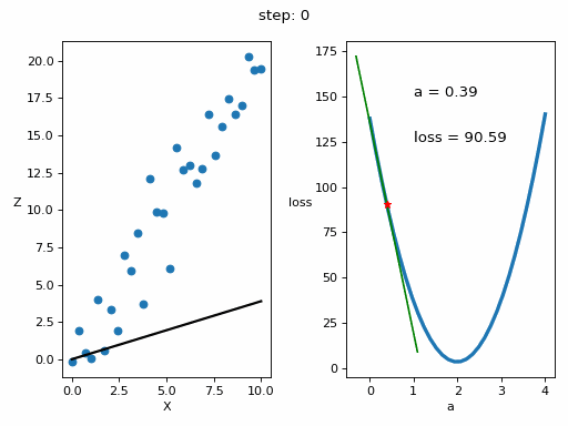
Let's represent the evolution of the training in a graph

	
		# Creamos GIF con la evolución del entrenamiento
 
from matplotlib.animation import FuncAnimation
from IPython.display import display, Image
 
# Creamos la gráfica inicial
fig, (ax1, ax2) = plt.subplots(1,2)
fig.set_tight_layout(True)
ax1.set_xlabel('X')
ax1.set_ylabel('Z  ', rotation=0)
ax2.set_xlabel('a')
ax2.set_ylabel('loss     ', rotation=0)
 
# Se dibujan los datos que persistiran en toda la evolución de la gráfica
ax1.scatter(x, z)
ax2.plot(posibles_a, perdidas, linewidth = 3)
 
# Se dibuja el resto de lineas que irán cambiando durante el entrenamiento
line1, = ax1.plot(x, Zs[0,:], 'k', linewidth=2) # Recta generada con la pendiente a aprendida
line2, = ax2.plot(Xs_linea_gradiente[0,:], Zs_linea_gradiente[0,:], 'g') # Gradiente de la función de error
punto2, = ax2.plot(As[0], Errores[0], 'r*') # Punto donde se calcula el gradiente
 
# Se dibujan textos dentro de la segunda figura del subplot
fontsize = 12
a_text = ax2.text(1, 150, f'a = {As[0]:.2f}', fontsize = fontsize)
error_text = ax2.text(1, 125, f'loss = {Errores[0]:.2f}', fontsize = fontsize)
 
# Se dibuja un título
titulo = fig.suptitle(f'step: {0}', fontsize=fontsize)
 
# Se define la función que va a modificar la gráfica con la evolución del entrenamiento
def update(i):
    # Se actualiza la linea 1. Recta generada con la pendiente a aprendida
    line1.set_ydata(Zs[i,:])
    
    # Se actualiza la linea 2. Gradiente de la función de error
    line2.set_xdata(Xs_linea_gradiente[i,:])
    line2.set_ydata(Zs_linea_gradiente[i,:])
 
    # Se actualiza el punto 2. Punto donde se calcula el gradiente
    punto2.set_xdata([As[i]])
    punto2.set_ydata([Errores[i]])
 
    # Se actualizan los textos
    a_text.set_text(f'a = {As[i]:.2f}')
    error_text.set_text(f'loss = {Errores[i]:.2f}')
    titulo.set_text(f'step: {i}')
 
    return line1, ax1, line2, punto2, ax2, a_text, error_text
 
# Se crea la animación con un refresco cada 200 ms
interval = 200 # ms
anim = FuncAnimation(fig, update, frames=np.arange(0, steps), interval=interval)
 
# Se guarda la animación en un gif
gif_name = "GIFs/entrenamiento_regresion.gif"
anim.save(gif_name, dpi=80, writer='pillow')
 
# Leer el GIF y mostrarlo
with open(gif_name, 'rb') as f:
    display(Image(data=f.read()))
 
# Se elimina la figura para que no se muestre en el notebook
plt.close()
	
	
		
	
	Copied

	
		&lt;IPython.core.display.Image object&gt;

We are going to explain the process again, but without focusing so much on each detail to reinforce the concepts.

We have the following values x and y

	
		x = np.array( [ 0. , 0.34482759, 0.68965517, 1.03448276, 1.37931034,
        1.72413793, 2.06896552, 2.4137931 , 2.75862069, 3.10344828,
        3.44827586, 3.79310345, 4.13793103, 4.48275862, 4.82758621,
        5.17241379, 5.51724138, 5.86206897, 6.20689655, 6.55172414,
        6.89655172, 7.24137931, 7.5862069 , 7.93103448, 8.27586207,
        8.62068966, 8.96551724, 9.31034483, 9.65517241, 10. ])
 
z = np.array( [-0.16281253, 1.88707606, 0.39649312, 0.03857752, 4.0148778 ,
        0.58866234, 3.35711859, 1.94314906, 6.96106424, 5.89792585,
        8.47226615, 3.67698542, 12.05958678, 9.85234481, 9.82181679,
        6.07652248, 14.17536744, 12.67825433, 12.97499286, 11.76098542,
       12.7843083 , 16.42241036, 13.67913705, 15.55066478, 17.45979602,
       16.41982806, 17.01977617, 20.28151197, 19.38148414, 19.41029831])
 
plt.scatter(x, z)
plt.xlabel('X')
plt.ylabel('Z  ', rotation=0)
plt.show()
	
	
		
	
	Copied

	
		&lt;Figure size 640x480 with 1 Axes&gt;

So we use a single neuron to try to find the line that best fits those points.

We just need to find the best possible value of a

We start by initializing a with a random value

	
		random.seed(45)
a = random.random()
a
	
	
		
	
	Copied

	
		0.2718754143840908

We calculate the z values generated by the neuron with the value of a that we just initialized.

	
		z_p = a*x
 
plt.scatter(x, z)
plt.plot(x, z_p, 'k')
plt.xlabel('X')
plt.ylabel('Z  ', rotation=0)
plt.show()
	
	
		
	
	Copied

	
		&lt;Figure size 640x480 with 1 Axes&gt;

But we see that with the value of a we have set, the neuron is not able to resemble the points.

We need to know how good or bad the value of a is, so we calculate the error of the neuron's output with respect to the data we have. For this, we use the mean squared error (MSE) using the formula

$loss = ∑i=1N ≤ft(zp-z\right)2N$

Right now, our error is

	
		error = loss(z, z_p)
error
	
	
		
	
	Copied

	
		103.72263739946467

Since we already have a way to measure the error, we want to decrease the error, so we look for the gradient of the error with respect to a to be zero, or as close to zero as possible. To achieve this, we perform a training loop in which we modify the value of a using the formula

$a' = a - α\partial loss\partial a$

Where $α$ is called the learning rate and determines the speed of learning.

	
		lr = 10**-3 # Tasa de aprendizaje o learning rate
steps = 100 # Numero de veces que se realiza el bucle de enrtenamiento
 
# Matrices donde se guardarán los datos para luego ver la evolución del entrenamiento en una gráfica
Zs = np.empty([steps, len(x)])
Xs_linea_gradiente = np.empty([steps, len(x_inicio)])
Zs_linea_gradiente = np.empty([steps, len(z_inicio)])
As = np.empty(steps)
Errores = np.empty(steps)
 
for i in range(steps):
    # Calculamos el gradiente
    dl = gradiente(a, x, z)
 
    # Corregimos el valor de a
    a = a - lr*dl
 
    # Calculamos los valores que obtiene la red neuronal
    z_p = a*x
 
    # Obtenemos el error
    error = loss(z, z_p)
 
    # Obtenemos las rectas de los gradientes para representarlas
    x_linea_gradiente, z_linea_gradiente = gradiente_linea(i_inicio, a=a, error=error, gradiente=dl)
 
    # Guardamos los valores para luego ver la evolución del entrenamiento en una gráfica
    As[i] = a
    Zs[i,:] = z_p
    Errores[i] = error
    Xs_linea_gradiente[i,:] = x_linea_gradiente
    Zs_linea_gradiente[i,:] = z_linea_gradiente
 
    # Imprimimos la evolución del entrenamiento
    if (i+1)%10 == 0:
        print(f"i={i+1}: error={error}, gradiente={dl}, a={a}")
	
	
		
	
	Copied

	
		i=10: error=28.075728775043547, gradiente=-61.98100236918255, a=1.1394358551489718
i=20: error=9.50524503591466, gradiente=-30.709631939506394, a=1.569284692740735
i=30: error=4.946395605365449, gradiente=-15.215654116766258, a=1.7822612353503635
i=40: error=3.8272482302958437, gradiente=-7.5388767490642445, a=1.887784395436304
i=50: error=3.552509863476323, gradiente=-3.7352756707945205, a=1.9400677933076504
i=60: error=3.4850646173147437, gradiente=-1.8507112931062708, a=1.9659725680580205
i=70: error=3.4685075514689503, gradiente=-0.9169690786711168, a=1.978807566971417
i=80: error=3.464442973977972, gradiente=-0.4543292594425819, a=1.9851669041474533
i=90: error=3.4634451649256888, gradiente=-0.22510581958202128, a=1.9883177551597053
i=100: error=3.463200213782052, gradiente=-0.111532834297016, a=1.989878902465877

We can see that the error has decreased significantly, from 103.72 that we had initially to 3.46 that we have now.

We represent the evolution of the training to see it graphically

Continue reading

Neural Networks: A Brief History, AI Winter, the 2012 Breakthrough, and the mainstream of 2022

Learn how neural networks work, their history since the 1950s, the AI Winter, and how ImageNet revolutionized AI in 2012. Beginner-friendly guide.

MCP Elicitation: Implementing Elicitation in Servers with FastMCP and Python

Learn how to implement elicitation in MCP (Model Context Protocol) servers with FastMCP. Complete step-by-step tutorial to create an intelligent travel booking agent that requests user information interactively. Includes server and client code, virtual environment setup with uv, and practical elicitation examples for real-time user data collection.

MCP Durability: Server and Client with Persistence for Long-Running Tasks

Learn to build durable MCP server and client for long-running tasks with persistence. Complete Model Context Protocol tutorial featuring SQLite data persistence, background task management, and real-time monitoring. Implement data migration, batch processing, and ML model training that survive server restarts. Python code examples using FastMCP, resources, tools, and durability patterns for enterprise applications.

Last posts -->

Have you seen these projects?

Horeca chatbot

Naviground

Subtify

View all projects -->

Do you want to apply AI in your project? Contact me!

Do you want to improve with these tips?

o1 prompt engineering

Create better prompts for o1 following an example

Memory profiler

See the memory usage of a script

DataLoader with pin_memory and num_workers

Increase DataLoader performance with pin_memory and num_workers

Last tips -->

Use this locally

Hugging Face spaces allow us to run models with very simple demos, but what if the demo breaks? Or if the user deletes it? That's why I've created docker containers with some interesting spaces, to be able to use them locally, whatever happens. In fact, if you click on any project view button, it may take you to a space that doesn't work.